ConvolutionalNeuralNetworksfor MalwareClassification · 2017-08-29 · convolutional neural...
100
Convolutional Neural Networks for Malware Classification Daniel Gibert Director: Javier Bejar Department of Computer Science A thesis presented for the degree of Master in Artificial Intelligence Facultat d’Informàtica de Barcelona (FIB) Facultat de Matemàtiques (UB) Escola Tècnica Superior d’Enginyeria (URV) Escola Politècnica de Catalunya (UPC) - BarcelonaTech Universitat de Barcelona (UB) Universitat Rovira i Virgili (URV) 20 October 2016
Transcript of ConvolutionalNeuralNetworksfor MalwareClassification · 2017-08-29 · convolutional neural...
Convolutional Neural Networks forMalware Classification
Daniel Gibert
Director: Javier BejarDepartment of Computer Science
A thesis presented for the degree of Master in ArtificialIntelligence
Facultat d’Informàtica de Barcelona (FIB)Facultat de Matemàtiques (UB)
Escola Tècnica Superior d’Enginyeria (URV)
Escola Politècnica de Catalunya (UPC) - BarcelonaTechUniversitat de Barcelona (UB)
Universitat Rovira i Virgili (URV)
20 October 2016

Abstract
According to AV vendors malicious software has been growing exponentiallylast years. One of the main reasons for these high volumes is that in orderto evade detection, malware authors started using polymorphic and meta-morphic techniques. As a result, traditional signature-based approaches todetect malware are being insufficient against new malware and the catego-rization of malware samples had become essential to know the basis of thebehavior of malware and to fight back cybercriminals.
During the last decade, solutions that fight against malicious software hadbegun using machine learning approaches. Unfortunately, there are few open-source datasets available for the academic community. One of the biggestdatasets available was released last year in a competition hosted on Kag-gle with data provided by Microsoft for the Big Data Innovators Gathering(BIG 2015). This thesis presents two novel and scalable approaches usingConvolutional Neural Networks (CNNs) to assign malware to its correspond-ing family. On one hand, the first approach makes use of CNNs to learn afeature hierarchy to discriminate among samples of malware represented asgray-scale images. On the other hand, the second approach uses the CNNarchitecture introduced by Yoon Kim [12] to classify malware samples accord-ing their x86 instructions. The proposed methods achieved an improvementof 93.86% and 98,56% with respect to the equal probability benchmark.
Acknowledgments
I would first like to thank my family, especially Mom, for the continuoussupport she has given me throughout my time in graduate school. Second,I would like to express my gratitude to my supervisor, Dr. Javier Béjar fortheir guidance during the course of this thesis.
1

Contents
1 Introduction 81.1 Objective . . . . . . . . . . . . . . . . . . . . . . . . . . . . . 121.2 Organization . . . . . . . . . . . . . . . . . . . . . . . . . . . 13
2 Background 142.1 Artificial Neural Networks . . . . . . . . . . . . . . . . . . . . 14
2.1.1 Perceptrons . . . . . . . . . . . . . . . . . . . . . . . . 152.1.2 Sigmoid neuron . . . . . . . . . . . . . . . . . . . . . . 162.1.3 Loss function . . . . . . . . . . . . . . . . . . . . . . . 162.1.4 Gradient Descent Algorithm . . . . . . . . . . . . . . . 172.1.5 Backpropagation . . . . . . . . . . . . . . . . . . . . . 19
2.2 Convolutional Neural Networks . . . . . . . . . . . . . . . . . 212.2.1 Local connectivity . . . . . . . . . . . . . . . . . . . . 222.2.2 Convolutional Layer . . . . . . . . . . . . . . . . . . . 222.2.3 Pooling Layer . . . . . . . . . . . . . . . . . . . . . . . 23
2.3 Overfitting . . . . . . . . . . . . . . . . . . . . . . . . . . . . . 252.3.1 Regularization . . . . . . . . . . . . . . . . . . . . . . . 252.3.2 Dropout . . . . . . . . . . . . . . . . . . . . . . . . . . 262.3.3 Artificially expanding the training data . . . . . . . . . 26
2.4 Deep Learning . . . . . . . . . . . . . . . . . . . . . . . . . . . 282.4.1 ReLU units . . . . . . . . . . . . . . . . . . . . . . . . 282.4.2 Gradient Descent Optimization Algorithms . . . . . . . 29
2

CONTENTS
3 State of the Art 33
4 Microsoft Malware Classification Challenge 394.1 What’s Kaggle? . . . . . . . . . . . . . . . . . . . . . . . . . . 394.2 Microsoft Malware Classification Challenge . . . . . . . . . . . 40
4.2.1 Bytes file . . . . . . . . . . . . . . . . . . . . . . . . . 414.2.2 ASM file . . . . . . . . . . . . . . . . . . . . . . . . . . 42
4.3 Winner’s solution . . . . . . . . . . . . . . . . . . . . . . . . . 464.4 Novel Feature Extraction, Selection and Fusion for Effective
Malware Family Classification . . . . . . . . . . . . . . . . . . 474.5 Deep Learning Frameworks . . . . . . . . . . . . . . . . . . . . 51
5 Learning Feature Extractors from Malware Images 535.1 Visualizing malware as gray-scale images . . . . . . . . . . . . 54
5.1.1 Malware families . . . . . . . . . . . . . . . . . . . . . 555.2 CNN Architectures . . . . . . . . . . . . . . . . . . . . . . . . 59
5.2.1 CNN A: 1C 1D . . . . . . . . . . . . . . . . . . . . . . 615.2.2 CNN B: 2C 1D . . . . . . . . . . . . . . . . . . . . . . 625.2.3 CNN C: 3C 2D . . . . . . . . . . . . . . . . . . . . . . 64
5.3 Results . . . . . . . . . . . . . . . . . . . . . . . . . . . . . . . 675.3.1 Evaluation . . . . . . . . . . . . . . . . . . . . . . . . . 675.3.2 Testing . . . . . . . . . . . . . . . . . . . . . . . . . . . 70
6 Convolutional Neural Networks for Classification of MalwareDisassembly Files 726.1 Representing Opcodes as Word Embeddings . . . . . . . . . . 74
6.1.1 Skip-Gram model . . . . . . . . . . . . . . . . . . . . . 756.2 Convolutional Neural Network Architecture . . . . . . . . . . 796.3 Results . . . . . . . . . . . . . . . . . . . . . . . . . . . . . . . 83
6.3.1 Evaluation . . . . . . . . . . . . . . . . . . . . . . . . . 836.3.2 Testing . . . . . . . . . . . . . . . . . . . . . . . . . . . 88
3
CONTENTS
7 Conclusions 907.1 Future Work . . . . . . . . . . . . . . . . . . . . . . . . . . . . 92
4
List of Figures
2.1 Effects of different learning rates . . . . . . . . . . . . . . . . . 182.2 AlexNet architecture . . . . . . . . . . . . . . . . . . . . . . . 212.3 Convolution . . . . . . . . . . . . . . . . . . . . . . . . . . . . 222.4 Max pooling . . . . . . . . . . . . . . . . . . . . . . . . . . . . 232.5 ReL and sigmoid functions comparison . . . . . . . . . . . . . 29
3.1 Most frequent 14 opcodes for goodware . . . . . . . . . . . . . 343.2 Most frequent 14 opcodes for malware . . . . . . . . . . . . . 343.3 Outline of Invencea’s Malware Detection Framework . . . . . . 363.4 Visualizing Malware as an Image . . . . . . . . . . . . . . . . 38
4.1 Malware Classification Challenge: dataset . . . . . . . . . . . 404.2 Snapshot of one bytes file . . . . . . . . . . . . . . . . . . . . 414.3 Snapshot of one assembly code file . . . . . . . . . . . . . . . 424.4 Top 10 opcodes in the training dataset . . . . . . . . . . . . . 444.5 Average of opcodes per malware family . . . . . . . . . . . . . 44
5.1 Visualizing Malware as a Gray-Scale Image . . . . . . . . . . . 545.2 Rammit samples . . . . . . . . . . . . . . . . . . . . . . . . . 555.3 Lollipop samples . . . . . . . . . . . . . . . . . . . . . . . . . 555.4 Kelihos_ver3 samples . . . . . . . . . . . . . . . . . . . . . . . 565.5 Vundo samples . . . . . . . . . . . . . . . . . . . . . . . . . . 565.6 Simda samples . . . . . . . . . . . . . . . . . . . . . . . . . . 56
5

LIST OF FIGURES
5.7 Tracur samples . . . . . . . . . . . . . . . . . . . . . . . . . . 575.8 Kelihos_ver1 samples . . . . . . . . . . . . . . . . . . . . . . . 575.9 Obfuscator.DCY samples . . . . . . . . . . . . . . . . . . . . . 575.10 Gatak samples . . . . . . . . . . . . . . . . . . . . . . . . . . . 585.11 Shallow Approach . . . . . . . . . . . . . . . . . . . . . . . . . 595.12 Overview architecture A: 1C 1D . . . . . . . . . . . . . . . . . 625.13 Overview architecture B: 2C 1D . . . . . . . . . . . . . . . . . 645.14 Overview architecture C: 3C 2D . . . . . . . . . . . . . . . . . 665.15 Approach A: CNNs training results . . . . . . . . . . . . . . . 68
6.1 Yoon Kim model architecture . . . . . . . . . . . . . . . . . . 736.2 Skip-gram model architecture . . . . . . . . . . . . . . . . . . 756.3 t-SNE representation of the word embeddings . . . . . . . . . 786.4 CNN Embedding layer output . . . . . . . . . . . . . . . . . . 806.5 CNN Convolutional layer output . . . . . . . . . . . . . . . . . 816.6 CNN Max-pooling & output layer . . . . . . . . . . . . . . . . 826.7 Heuristic Search: Learning Rate . . . . . . . . . . . . . . . . . 846.8 Heuristic Search: Embedding size . . . . . . . . . . . . . . . . 846.9 Heuristic Search: #Filters . . . . . . . . . . . . . . . . . . . . 856.10 Heuristic Search: Filter Sizes . . . . . . . . . . . . . . . . . . . 866.11 Approach B: CNNs training results . . . . . . . . . . . . . . . 87
6

List of Tables
4.1 Number of samples per class with 0 instructions . . . . . . . . 454.2 Winner’s solution: confusion matrix . . . . . . . . . . . . . . . 474.3 List of feature categories and their evaluation in XGBoost . . 49
5.1 CNN 1C 1D: confusion matrix . . . . . . . . . . . . . . . . . . 685.2 CNN 2C 1D: confusion matrix . . . . . . . . . . . . . . . . . . 695.3 CNN 3C 2D: confusion matrix . . . . . . . . . . . . . . . . . . 69
6.1 CNN without pretrained word embeddings: confusion matrix . 876.2 CNN with pretrained word embeddings: confusion matrix . . . 886.3 Approach B: Test scores . . . . . . . . . . . . . . . . . . . . . 88
7
Chapter 1
Introduction
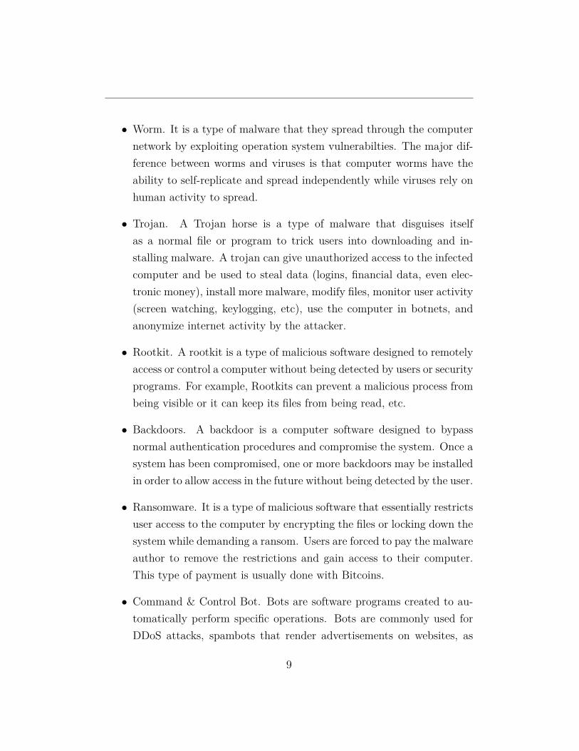
Malware, short for malicious software, refers to software programs designedto damage or do any kind of unwanted actions on a computer system such asdisrupting computer operations, gather sensitive information, bypass accesscontrols, gain access to private computer systems and display unwanted ad-vertising. Malware can be divided into the following categories not mutuallyexclusive depending on their purpose.
• Adware. It is a type of malware that automatically delivers adver-tisements. Advertising-supported software often comes bundled withsoftware and applications and most of them serve as a revenue tool.
• Spyware. It is a type of malware that spies and track user activity with-out their knowledge. The capabilities of spyware can include keystrokescollection, financial data harvesting or activity monitoring.
• Virus. A virus is a type of malicious software capable of copying itselfand spreading to other computers. Viruses can spread through emailattachments, through the network the computer is connected if anyother computer inside the network has been infected, by downloadingsoftware from malicious sites, etc.
8
• Worm. It is a type of malware that they spread through the computernetwork by exploiting operation system vulnerabilties. The major dif-ference between worms and viruses is that computer worms have theability to self-replicate and spread independently while viruses rely onhuman activity to spread.
• Trojan. A Trojan horse is a type of malware that disguises itselfas a normal file or program to trick users into downloading and in-stalling malware. A trojan can give unauthorized access to the infectedcomputer and be used to steal data (logins, financial data, even elec-tronic money), install more malware, modify files, monitor user activity(screen watching, keylogging, etc), use the computer in botnets, andanonymize internet activity by the attacker.
• Rootkit. A rootkit is a type of malicious software designed to remotelyaccess or control a computer without being detected by users or securityprograms. For example, Rootkits can prevent a malicious process frombeing visible or it can keep its files from being read, etc.
• Backdoors. A backdoor is a computer software designed to bypassnormal authentication procedures and compromise the system. Once asystem has been compromised, one or more backdoors may be installedin order to allow access in the future without being detected by the user.
• Ransomware. It is a type of malicious software that essentially restrictsuser access to the computer by encrypting the files or locking down thesystem while demanding a ransom. Users are forced to pay the malwareauthor to remove the restrictions and gain access to their computer.This type of payment is usually done with Bitcoins.
• Command & Control Bot. Bots are software programs created to au-tomatically perform specific operations. Bots are commonly used forDDoS attacks, spambots that render advertisements on websites, as
9

web spiders or for distributing malware. One way to defend againstbots is by using CAPTCHA tests in websites to verify users as human.
Nowadays, the detection of malicious software is done mainly with heuristicand signature-based methods that struggle to keep up with malware evolu-tion. Signature-based methods haven been heavily used for antivirus softwarefor decades. A malware signature is an algorithm or hash that uniquely iden-tifies a specific virus. While identifying a particular virus is advantageousit is quicker to detect a virus family through a generic signature. Virus re-searchers found that all viruses in a family share common behaviors and asingle generic signature can be created for them. However, malware authorsalways try to stay a step ahead of AV software by writing polymorphic andmetamorphic malware to do not match virus signatures. On one hand, poly-morphic code uses a polymorphic engine to mutate while keeping the originalalgorithm intact. Encryption is the most common way to hide code. On theother hand, metamorphic viruses translate their own binary code into a tem-porary representation, editing the temporary representation of themselvesand then translate the edited form back to machine code again. This muta-tion can be done by using techniques such as changing what registers to use,changing machine instructions to equivalent ones, inserting NOP instructionsor reordering independent instructions.
Therefore, AV vendors rely also in heuristic-based methods. This approachis based on rules determined by experts which rely on dynamic analysis ofmalicious behavior and thus, it can deal with unknown malware but it alsogenerates greater amounts of false positives than signature-based methodsbecause not each one of the detected suspicious executable files is a malwarefile. As a result, AV vendors attempted to use an hybrid analysis approachby using both signature-based and heuristic-based methods to tackle withunknown malware. In contrast, before creating the signatures for malware,it has first to be analyzed so to understand its capabilities and behavior. The
10

program capabilities and behavior can be observed either by examining itscode or by executing it in a safe environment.
1. Static Analysis. It refers to the analysis of a program without executingit. The patterns detected in this kind of analysis include string signa-ture, byte-sequence or opcodes frequency distribution, byte-sequencen-grams or opcodes n-grams, API calls, structure of the disassembledprogram, etc. The malicious program is usually unpacked and de-cripted before doing static analysis by using disassembler or debuggertools such as IDA Pro or OllyDbg which can be used to reverse com-piled Windows executables and display malware code as a sequence ofIntel x86 assembly instructions.
2. Dynamic Analysis. It refers to the analysis of the behavior of a ma-licious program while it is being executed in a controlled environment(virtual machine, emulator, sandbox, etc). The behavior is monitoredby using tools like Process Monitor, Process Explorer, Wireshark orCapture BAT. This kind of analysis tries to monitor function and APIcalls, the network, the flow of information, etc. Compared to staticanalysis, it is more effective and does not require the executable to bedisassembled but on the other hand, it takes more time and consumesmore resources than static analysis, being more difficult to scale. Inaddition, as the controlled environment in which the malware is moni-tored is different from the real one the program may behave different.That’s because some behavior of malware might be triggered only un-der certain conditions such as via a specific command or on a specificsystem date and in consequence, can’t be detected in a virtual environ-ment
In recent years, the possibility of success of machine learning approaches hasincreased thanks to the confluence of three developments: (1) the rise ofcommercial feeds that provide volumes of new malware, (2) the computing
11
1.1. OBJECTIVE
power has become cheaper meaning that researchers can fit large and morecomplex models to data and (3) machine learning as discipline has evolvedand there are more tools at their disposal. Machine learning approaches holdthe promise that they might achieve high detection rates without the needof human signature generation required by traditional approaches. In con-sequence, AV companies and researchers begun to employ machine learningclassifiers to help them address this problem such as logistic regression[22],neural networks[8] and decision trees[14].
The two principal tasks that have been carried out within the scope of mal-ware analysis are (1) malware detection and (2) malware classification. First,a file needs to be analyzed to detect if has any malicious content. In caseit exhibits any malicious content it is assigned to the most appropriate mal-ware family according to their content and behavior through a classificationmechanism.
1.1 Objective
This master thesis aims to explore the problem of malware classification. Inparticular, this thesis proposes two novel approaches based on ConvolutionalNeural Networks (CNNs). On one hand, CNNs were applied for learningdiscriminative patterns from malware images based on the work performed byNataraj et al.[21]. On the other hand, the CNN architecture proposed in [12]was used to classify malicious software based on malware’s x86 instructions.Both approaches have been evaluated on the data provided by Microsoft forthe BIG Cup 2015 (Big Data Innovators Gathering).
12

1.2. ORGANIZATION
1.2 Organization
The thesis is organized following chapters. The first and current chapter isthe introduction, which also contains the objectives and the organization ofthe thesis. The second chapter introduces the background of the project,focusing on neural networks and deep learning from its beginning until now.The third chapter presents the state of the art review with special attentionon the machine learning algorithms and features used to detect and classifymalware. The fourth chapter introduces the Kaggle platform and the Mi-crosoft’s Malware Classification Challenge. In addition, it also describes twosolutions of the competition. The fifth chapter describes the approach basedon the representation of malware as gray-scale images and the sixth chapterexplains how Convolutional Neural Networks can be used to extract featuresfrom malware’s x86 instructions represented via word embeddings. Finally,the last chapter wraps up the conclusions and the future work to be done.
13
Chapter 2
Background
Nowadays Deep Learning is the hottest topic in the Artificial Intelligenceand Machine Learning field. Deep Learning refers to the set of techniquesused for learning in Neural Networks with many layers. However, it is basedon a set of previous ideas that appeared over the 60s. In this chapter areexplained the most important concepts behind deep learning.
2.1 Artificial Neural Networks
Artificial Neural Networks are a family of models inspired by the way biolog-ical nervous systems, such as the brain, process information which enables acomputer to learn from data. There are different types of NNs but in thisthesis are only presented two of them: (1) feed-forward networks and (2)convolutional neural networks. First it is introduced the architecture of afeed-forward network. Thus, this type of nets are composed by at least threelayers, one input layer, one output layer and one or more hidden layers. Afeed-forward network has the following characteristics:
• Neurons are arranged in layers, with the first layer taking in inputs andthe last layer producing the output.
14

2.1. ARTIFICIAL NEURAL NETWORKS
• Each neuron in one layer is connected to every neurons in the nextlayer.
• There is no connection between neurons in the same layer.
To understand how a neural network works, first it has to be understoodwhat are neurons, how neurons learn and how the information pass from oneneuron to another.
2.1.1 Perceptrons
A perceptron was the earliest supervised learning algorithm and it is thebasic building block of Artificial Neural Networks (ANN). It was first intro-duced in 1957 at the Cornell Aeronautical Laboratory by Frank Rosenblatt.
It works by taking several inputs (x1, x2, ..., xj) and producing a single output(y). Rosenblat introduced weights (w1, w2, ..., wj) to express the importanceof the respective inputs to the output. The output of the perceptron is either0 or 1 and it is determined by whether the weighted sum ∑
j wj ∗ xj + b isless than or greater than 0.
output =
1 : if w ∗ x+ b > 0
0 : if w ∗ x+ b <= 0
However, a perceptron can only output zero or one, making impossible toextend the model to work on classification tasks with multiple categories.This issue can be solved by having multiple perceptrons in a layer, such thatall these perceptrons receive the same input and each one is responsible forone output of the function. In fact, Artificial Neural Networks (ANNs) arenothing more than layers of perceptrons (neurons or units as called nowa-days). A perceptron can be seen as an ANN with only one layer, the outputlayer, with 1 neuron.
15

2.1. ARTIFICIAL NEURAL NETWORKS
2.1.2 Sigmoid neuron
The main limitation of perceptrons is that there are very difficult to tune,because minimum changes in the weights and bias of any single perceptroncan cause the output to change drastically by completely flip, from 0 to 1 orviceversa. And if we have a network of perceptrons, a single flip can com-pletely change the behavior of the rest of the network.This problem was solved by the introduction of the sigmoid neuron.
Exactly as the perceptron, a sigmoid neuron has inputs (x1, x2, ..., xj) andit also has weights for each input and a bias, but the output can be a realnumber. The sigmoid function is defined as:
σ(z) = 11 + e−z
And the output of the sigmoid neuron is:
11 + exp(−∑
j wj ∗ xj − b)
Hence, the only difference between the perceptron and the sigmoid neuron isthe activation function.
2.1.3 Loss function
To measure the performance of the neural network it is defined a function,typically named cost or loss function which given a prediction or set of pre-dictions and a label or a set of labels measures the discrepancy between thealgorithms prediction and the correct label. There are various cost functionsbut the most common and simple in neural networks is the mean squarederror (MSE).
16

2.1. ARTIFICIAL NEURAL NETWORKS
The mean squared error can be defined as:
L(W, b) = 1/m(m∑
i=1||h(xi)− yi||2)
where:
• m is the number of training examples
• xi is the ith training sample
• yi is the class label for the ith training sample
• h(xi) is the algorithm’s prediction for the ith training sample
The goal in training neural networks is to find weights and biases that min-imizes some cost/loss function C. For that, it is used an algorithm calledgradient descent.
2.1.4 Gradient Descent Algorithm
Gradient Descent is an algorithm for minimizing the loss function. It is usedto find the local minimum of the loss function. Next you will find an outlineof the algorithm.
1. Start with a random initialization of each weight and bias in the NN. Itis important to randomly initialize all parameters because if not, if allparameters start off at identical values, then all the hidden layer unitswill end up learning the same function of the input. In consequence,random initialization serves the purpose of symmetry breaking.
2. Keep iterating to update the parameters W,b as follows until it hope-fully ends up at a minimum:
W li,j = W l
i,j − α∂
∂W li,j
L(W, b)
17

2.1. ARTIFICIAL NEURAL NETWORKS
bli = bl
i − α∂
∂bli
L(W, b)
where α is the learning rate and W li,j and bl
i denote each weight andbias in a particular layer l in the NN, respectively.
The derivative of the overall loss function can be computed as:
∂
∂W li,j
L(W, b) = [ 1m
m∑i=1
∂
∂W li,j
L(W, b : xi, yi)]
∂
∂bli
L(W, b) = [ 1m
m∑i=1
∂
∂bli
L(W, b : xi, yi)]
The learning rate is used to control how big a step is taken downhill withgradient descent. Selecting the correct learning rate is critical. On one hand,if α is too small, gradient descent can be slow. On the other hand, if α istoo large, gradient descent can overstep the minimum and even diverge.
Figure 2.1: Effects of different learning rates
18

2.1. ARTIFICIAL NEURAL NETWORKS
2.1.5 Backpropagation
The key step is to compute all those partial derivates presented before. There-fore, to compute efficiently these partial derivates is used the backpropagationalgorithm.
The intuition behind is as follows. Given a training example (xi, yi) firstof all it is ran a forward pass to compute all the activations through thenetwork (also the output value of the hypothesis h(xi)). Thus, for each nodei in layer l it is computed an error term, δl
i, that measures how much thatnode was responsible for any errors in the output. For an output node, theerror term is measured directly from the difference between the network’sactivation and the true target value and is defined as δnl
i , where nl is the out-put layer. For hidden units, it is computed δl
i based on the weighted averageof the error terms of the nodes that use al
i as an input (ali = activation of
node i in layer l).
Overview of the algorithm:
1. Compute the activation of the layers l1, l2 and so on up to the outputlayer lnl by performing a feedforward pass.
2. For each output unit i in layer nl compute the error term δnli .
δnli = ∂
∂znli
∗ 12 ||y − hW,b(x)||2
3. For all hidden layers l = nl − 1, nl − 2, ..., 2. Compute for each node iin layer l:
δli =
l+1∑j=1
W ljiδ
l+1j
∗ f ′(zli)
19

2.1. ARTIFICIAL NEURAL NETWORKS
4. Finally, compute the desired derivatives given as:
∂
∂W li,j
L(W, b : x, y) = alj ∗ δl+1
i
∂
∂bli
L(W, b : x, y) = δl+1i
20

2.2. CONVOLUTIONAL NEURAL NETWORKS
2.2 Convolutional Neural Networks
A Convolutional Neural Network (CNN) is a type of feed-forward NN inwhich the connectivity pattern between its neurons is inspired by the orga-nization of the animal visual cortex, whose individual neurons are arrangedin such a way that they respond to overlapping regions tilling the visual field.
CNN are composed by three types of layers: (1) fully-connected, (2) con-volutional (3) and pooling. All the various implementations of CNN can beloosely described as involving the following process:
1. Convolve several small filters on the input image.
2. Subsample this space of filter activations.
3. Repeat steps 1 and 2 until you are left with enough high level features.
4. Apply a standard feed-forward NN to the resulting features.
Figure 2.2: AlexNet architecture
Figure 2.2 corresponds to the architecture used in [16] that was applied tothe ImageNet classification contest. The architecture consists of 8 learnablelayers, the first five are convolutional and the rest are fully-connected layers.
21

2.2. CONVOLUTIONAL NEURAL NETWORKS
2.2.1 Local connectivity
It is impractical to connect neurons to all neurons in the previous layer whendealing with high-dimensional inputs like images because in such networkarchitectures the spatial structure of the data is not taken into account.In convolutional neural networks each neuron is connected to a small re-gion of the input neurons (each neuron connects only to a small contiguousregion of pixels in the input) and thus, CNNs are able to exploit spatiallylocal correlation by enforcing a local connectivity pattern between neuronsof adjacent layers.
2.2.2 Convolutional Layer
Convolutional layers are the core of a CNN. A convolutional layer consists of aset of learnable kernels which are convolved across the width and the heightof the input features during the forward pass producing a 2-dimensionalactivation map of the kernel.As a summary, a kernel consists of a layer of connection weights with theinput being the size of a small 2D patch and the output being a single unit.
Figure 2.3: Convolution
In figure 2.3 it is represented how convolution works. Considering an im-age of 5x5 pixels as in the figure, where 0 means values completely black and255 means completely white. In the center of the figure, it has been defineda kernel of 3x3 pixels with all eight 0 except one wright set at 1. The outputis the result of computing the kernel at each possible position in the image.
22

2.2. CONVOLUTIONAL NEURAL NETWORKS
Whether or not the kernel is convolved through all positions it is determinedby the stride. For example, for stride 1, it outputs the typical convolutionbut for stride 2 half of the convolutions are avoided because there should be2 pixels of distance between centers.
The size of the output after convolving a kernel of size Z over an imageN with stride S is defined as:
output = N − ZS
+ 1
2.2.3 Pooling Layer
Pooling is a form of non-linear down-sampling. There are several non-linearfunctions to implement pooling such as the minimum, the maximum andthe average but the most common is the maximum. Max pooling works bypartitioning the image into a set of non-overlapping rectangles and for eachsub-region outputs the maximum value.
Figure 2.4: Max pooling
The main benefits of max-pooling are:
1. It reduces computation for upper layers by eliminating non-maximalvalues.
23

2.2. CONVOLUTIONAL NEURAL NETWORKS
2. It provides a form of translation invariance and in consequence, pro-vides additional robustness to position being a way of reducing thedimensionality of intermediate representations.
24

2.3. OVERFITTING
2.3 Overfitting
Overfitting refers to the condition a predictive model describes the randomnoise of a particular data instead of learning the underlying relationship. Asa result, these models may not yield accurate predictions for new observa-tions.
This section describes the most common techniques used to avoid overfit-ting in large networks.
2.3.1 Regularization
Regularization adds an extra term, named regularization term to the lossfunction in a way that in consequence, the network would prefer to learn smallweights and penalize large weights. Regularization usually doesn’t affectbiases. That’s because large biases make it easier for neurons to saturate,which is sometimes desirable. Moreover, having large biases doesn’t make aneuron sensitive to its inputs in the same way as having large weights.
• L2 regularization.
L(W, b) = L(W, b)0 + λ
2n∑w
w2
• L1 regularization.
L(W, b) = L(W, b)0 + λ
n
∑w
|w|
where L(W, b)0 is the original unregularized loss function.
25

2.3. OVERFITTING
2.3.2 Dropout
In large neural networks, it is difficult to average the predictions of differentnetworks at test time. To address this problem, dropout was introduced in[32] by Geoffrey Hinton. The idea behind is to randomly drop units (alongwith their connections) from the neural network during training to preventneurons from co-adapting too much.
At each iteration, we randomly and temporaly disconnect a percentage ofthe hidden neurons (usually, half of them) in the network except those inthe input and the output layer. After that, the input is propagated throughthe modified network and then the result is backpropagated also through themodified network. After updating the appropiate weights and biases, theprocess is repeated by, first restoring the dropout neurons, then choosing anew random subset of hidden neurons to disconnect and so on.
Heuristically, the result of dropout is like training different neural networksand in consequence, the dropout procedure is like averaging the effects of alarge number of networks. These networks will overfit in different ways butat the end, hopefully, the network effect of dropout will be to reduce over-fitting. Lastly, by reducing neurons co-adaptations, a neuron cannot relyon the presence of a particular other neuron and is forced to learn more ro-bust features that are useful in conjunction with the other different randomsubsets of neurons.
2.3.3 Artificially expanding the training data
One of the best ways of reducing overfitting is to increase the size of thetraining data. Unfortunately, training data sometimes is expensive or difficultto acquire. To attach this problem, training data can be artificially expanded.In particular, in recent competitions such as CIFAR-10, training images were
26

2.3. OVERFITTING
cropped, flipped and transposed in various ways to expand the training data.
27

2.4. DEEP LEARNING
2.4 Deep Learning
As defined at the beginning of the chapter, deep learning is the term usedto describe the techniques used to learn in networks with many layers (deepneural networks). What convert a neural network into a deep neural networkis basically the number of layers. However, if deep neural networks are just aNN with more layers, why it has been until recently that they have attractedthat much attention? Well, it is mainly because of two reasons: (1) thecomputational power needed to train this networks and (2) the vanishinggradient problem.
1. The basic idea of software able to simulate the neocortex’s neuronsin an artificial neural network is decades old but because of the im-provements in mathematical formulas and the increasingly powerfulcomputers, computer scientist have been able to model networks withmany more layers than before.
2. The vanishing gradient problem was introduced in [10] by Sepp Hochre-iter which found that in a neural network with activation functions suchas the sigmoid or the hyperbolic tangent where the gradient range is(−1, 1) or [0, 1), backpropagation is computed by the chain rule, multi-plying n of this small numbers from the output layer through a n-layernetwork, meaning that gradient decreased exponentially with n. Thisresults in the front layers training much more slowly than other layers.
2.4.1 ReLU units
The vanishing gradient problem was not solved until 2010 by the introductionof the Rectified Linear units (ReLU) [9]. The activation function of ReLUunits is defined as:
f(x) =∞∑
i=1σ(x− i+ 0.5) ≈ log(1 + ex)
28

2.4. DEEP LEARNING
The softmax function log(1 + ex) can be approximated by the max functionor hard-max function f(x) = max(0, x).
Figure 2.5 presents a graphically comparison between the ReL and the sig-moid function.
Figure 2.5: ReL and sigmoid functions comparison
The main difference between both functions is that:
• The sigmoid function has range [0, 1] while the ReL function has range[0,∞).
• The gradient of the sigmoid function vanishes as it is increased or de-creased x while the gradient of the ReL function doesn’t vanish as x isincreased.
2.4.2 Gradient Descent Optimization Algorithms
There are three variants of the gradient descent algorithm, which differ inhow much data is used to compute the gradient of the objective function.
29

2.4. DEEP LEARNING
1. Batch Gradient Descent. It computes the gradients for the loss functionL(W,b) for the entire training set. It guarantees the convergence to theglobal minimum for convex error surfaces and to a local minimum fornon-convex surfaces.
2. Stochastic Gradient Descent. It performs a parameter update for eachtraining example xi and label yi. It is used for online learning as itperforms one update at a time. It enables to jump to new and potentialbetter local minimum but complicates the convergence to the exactlocal minimum.
3. Mini-batch Gradient Descent[17]. It computes the gradients for theloss function L(W,b) only for a small batch of n training samples. Itsfaster than batch gradient descent and leads to a better convergencethan stochastic gradient descent.
Next it is presented an outline of some algorithms used in deep learning tooptimize the gradient descent algorithm.
1. Momentum [25]The simplest gradient algorithm known as steepest descent 2.1.4, mod-ifies the weight at time step t according to:
W li,j = W l
i,j − α∂
∂W li,j
L(W, b)
bli = bl
i − α∂
∂bli
L(W, b)
However, it is known that learning such scheme can be very slow. Toimprove the speed of convergence of the gradient descent algorithm itis included the momentum term in the formula:
W li,j,t+1 = W l
i,j,t − α∂
∂W li,j
L(W, b) + γW li,j,t−1
30

2.4. DEEP LEARNING
bli,t+1 = bl
i,t − α∂
∂bli
L(W, b) + γbli,t
where γ is the momentum term. In consequence, the modification ofthe weight vector at the step t depends on both the current gradientand the weight change of the step t− 1.
2. Adagrad [5]Adagrad is an algorithm for gradient-based optimization that adaptsthe learning rate to the parameters, performing smaller updates forfrequent parameters and larger updates for infrequent parameters.Adagrad uses a different learning rate for every parameterW l
i,j,t at eachtime step t. In its update rule, it modifies the general learning rate α ateach time step t for every parameter W l
i,j,t based on the past gradientsthat have been computed for W l
i,j,t.
W li,j,t+1 = W l
i,j,t −α
Glt,ij + ε
∗ ∂
∂W li,j
L(W, b)
where Glt,ij ∈ Rdxd is the diagonal matrix where each diagonal element
ij is the sum of the squares of the gradients W li,j,t+1 up to time step t 24
and ε is smoothing term that avoids division by zero (≈ 1e− 8).
3. Adam [13]Adam is the acronym for Adaptive Moment Estimation. It is anothermethod that computes adaptive learning rates for each parameter. Itstores an exponentially decaying average of the past squared gradientsthat we will denota vt and similar to momentum, it keeps an exponen-tially decaying average of past gradients mt:
mt = β1mt−1 + (1− β1) ∗ gtvt = β2vt−1 + (1− β2) ∗ g2t
and gt is the gradient of the objective function and β1 and β2 are thedecay rates. mt and vt are the estimates of the first moment or mean
31

2.4. DEEP LEARNING
and the second moment or uncentered variance of the gradients, respec-tively. mt and vt are initialized as vectors of 0’s and in consequence,during initial time steps and when the decay rates are small they tendto be biased towards 0. To solve this problem, they computed thebias-corrected first and second moment estimates:
m̂t = mt
1− βt1v̂t = vt
1− βt2
As a result, the Adam update rule is defined as:
Wt+1 = Wt −α√v̂t + ε
∗ m̂t
32
Chapter 3
State of the Art
During the last decade, researchers and anti-virus vendors have begun em-ploying machine learning algorithms like the Association Rule, Support Vec-tor Machines, Random Forests, Naive Bayes and Neural Networks to addressthe problem of malicious software detection and classification. An overviewof the methods can be found in [26], [7] and [6]. Following a few of theseapproaches used in literature are discussed.
1. Byte-sequence N-grams[33, 31]The representation of a malware file as a sequence of hex values can beeffectively described through n-gram analysis. A N-gram is a contigu-ous sequence of n hexadecimal values from a given malware file. Eachelement in the byte sequence can take one out of 257 different values,i.e. the 256 byte range plus the special ‘??’ symbol. Byte-sequenceN-grams were first presented in [33], where they proposed a N-grambased algorithm for malware classification implemented in IBM’s an-tivirus scanner. The algorithm used 3-grams as features and a neuralnetwork as a classification model. Notice that the size of the featuresincrease exponentially being 2562 for a bigram model and 2563 for a tri-gram model being the techniques for dimensionality reduction a mustin this kind of models.
33

2. Opcodes N-grams [11, 27, 2, 3, 30]Similar to byte-sequence N-grams, n-gram models have been generatedfrom opcodes extracted from assembly language code files. An opcode(abbreviated from operation code) is the portion of a machine languageinstruction that specifies the operation to be performed. In particular,[3] investigated the most frequent opcodes and the rare opcodes presentin both goodware and malware. The following two charts show the 14most frequent opcodes in goodware and in malware, respectively.
Figure 3.1: Most frequent 14 opcodes for goodware
Figure 3.2: Most frequent 14 opcodes for malware
3. Portable Executable [37, 28]PE format is a file format for executables, DLLs and object code com-
34

monly used in the Windows operating systems. PE format is a dataformat that encapsulates the necessary information for the WindowsOS loader to manage the executable code. It includes information suchas dynamic library references for linking and API import and exporttables.
Features from Portable Executables (PE) are extracted by perform-ing static analysis using structural information of PE and are usefulto indicate whether or not the file has been manipulated or infectedto perform malicious activity. In [37] they extracted the following fea-tures from PE: (1) File pointers which denote the position within thefile as it is stored on disk; (2) Import sections which describe functionsfrom which DLLs were used and the list of DLLs of the executablethat are imported; (3) Exports section which describes the functionsthat are exported; (4) Structure of the PE header such as features likethe code and file size, the creation time, etc. After the feature extrac-tion process they build an ensemble of support vector machines. Thetraining set consisted of 9838 executables, from which 2320 were be-nign executables, 1936 backdoors, 1769 spyware, 1911 trojans and 1902worms. They tested the performance of the classifier on two datasets:(1)Malfease and (2)VXheavens.
In [28], Invencea Labs build a Deep Neural Network to detect malwareby using a set of features derived from the numerical fields extractedfrom the file binary’s PE packaging. The Deep NN consisted of threelayers: the input layer of 1024 input features and two hidden layers of1024 PReLU units each one. The output layer consisted of one sigmoidunit denoting whether the file is goodware or malware. In the followingpicture you can see an outline of the framework.
35

Figure 3.3: Outline of Invencea’s Malware Detection Framework
4. Entropy [29, 18]Malware authors use obfuscation techniques to pass through signature-based detection systems of antivirus programs. For this reason, it isexamined the statistical variation in malware samples to identify packedand encrypted samples. In [18] it was presented a tool to analyze theentropy of each PE section in order to determine which executablesections might be encrypted or packed. They found that the averageentropy is 4.347, 5.099, 6.801, 7.175 for plain files, native executables,packed executables and encrypted executables, respectively.
5. API calls [4, 36]API and function calls have been widely used to detect and classifymalicious software. An experiment was conducted to determine thetop maliciously used APIs. They retrieved the imports of all of the PEfiles and proceeded to count the number of times each sample uniquelyimported an API. They found that there was a total of 120126 uniquelyimported APIs.
In [4] they proposed a malware detection system which uses Window
36

API call sequences. They used a 3rd order Markov chain, i.e. 4-grams,to model the API calls. The malicious executables mainly consisted ofbackdoors, worms and Trojan horses collected from VXHeavens. Theirdetection system achieved an accuracy of 90%.
6. Use of registersIn [19], they proposed a method based on similarities of binaries behav-iors. They assumed that the behavior of each binary can be representedby the values of memory contents in its run-time. In other words, valuesstored in different registers while malicious software is running can bea distinguishing factor to set it apart from those of benign programs.Then, the register values for each API call are extracted before andafter API is invoked. After that, they traced the changes of registersvalues and created a vector for each of the values of EAX, EBX, EDX,EDI, ESI and EBP registers. Finally, by comparing old and unseenmalware vectors they achieved an accuracy of 98% in unseen samples.
7. Call GraphsA call graph is a directed graph that represents the relationships be-tween subroutines in a computer program. In particular, each noderepresents a procedure/function and each edge (f,g) indicates that pro-cedure f call procedure g. This kind of analysis have been used formalware classification with good results. In [15], they presented aframework which builds a function call graph from the informationextracted from disassembled malware programs. For every node (i.e.function) in the graph, they extracted attributes including library APIscalls and how many I/O read operations have been been made by thefunction. Then, they computed the similarity between any two mal-ware instances.
37
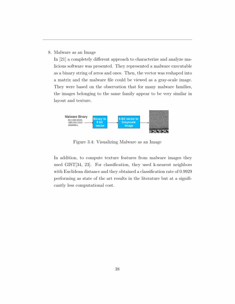
8. Malware as an ImageIn [21] a completely different approach to characterize and analyze ma-licious software was presented. They represented a malware executableas a binary string of zeros and ones. Then, the vector was reshaped intoa matrix and the malware file could be viewed as a gray-scale image.They were based on the observation that for many malware families,the images belonging to the same family appear to be very similar inlayout and texture.
Figure 3.4: Visualizing Malware as an Image
In addition, to compute texture features from malware images theyused GIST[34, 23]. For classification, they used k-nearest neighborswith Euclidean distance and they obtained a classification rate of 0.9929performing as state of the art results in the literature but at a signifi-cantly less computational cost.
38
Chapter 4
Microsoft MalwareClassification Challenge
The content of this chapter is structured as follows. First of all, it is presentedthe Microsoft Malware Classification Challenge and the platform where thecompetition was hosted. Secondly, it is described the winner’s solution of thechallenge and the set of techniques they used to win the competition followedby an approach that achieved a logloss of 0.0064 and used features extractedfrom gray-scale images of malware. Lastly, it is presented the deep learninglibrary used to implement the neural networks.
4.1 What’s Kaggle?
Kaggle is a platform where a large community of data scientist comprisedfrom thousands of MsCs and PhDs from fields such as computer science,statistics and maths compete to solve valuable problems. These problemscome from competitions that companies host in Kaggle or from competitionsthat are part of class homework or projects in academic institutions.
39

4.2. MICROSOFT MALWARE CLASSIFICATION CHALLENGE
4.2 Microsoft Malware Classification Challenge
In 2015, Microsoft hosted a competition in Kaggle with the goal of classifyingmalware into their respective families based on the their content and charac-teristics. For this challenge, Microsoft provided a dataset of 21741 samples,with 10868 for training and the other 10873 for testing, being a dataset ofalmost half a terabyte uncompressed. Microsoft provided a set of malwaresamples representing 9 different malware families. Each malware sample hadan Id, a 20 character hash value uniquely identifying the sample and a class,an integer representing one of the 9 malware family names to which the mal-ware belong: (1) Ramnit, (2) Lollipop, (3) Kelihos_ver3, (4) Vundo, (5)Simda, (6) Tracur, (7) Kelihos_ver1, (8) Obfuscator.ACY, (9) Gatak. Thedistribution of classes present in the training data is not uniform and thenumber of instances of some families significantly outnumbers the instancesof other families.
Figure 4.1: Malware Classification Challenge: dataset
For each observation we were provided with a file containing the hexadec-
40
4.2. MICROSOFT MALWARE CLASSIFICATION CHALLENGE
imal representation of the file’s binary content and a file containing metadatainformation extracted from the binary content, such as function calls, strings,sequence of instructions and registers used, etc, that was generated using theIDA disassembler tool.
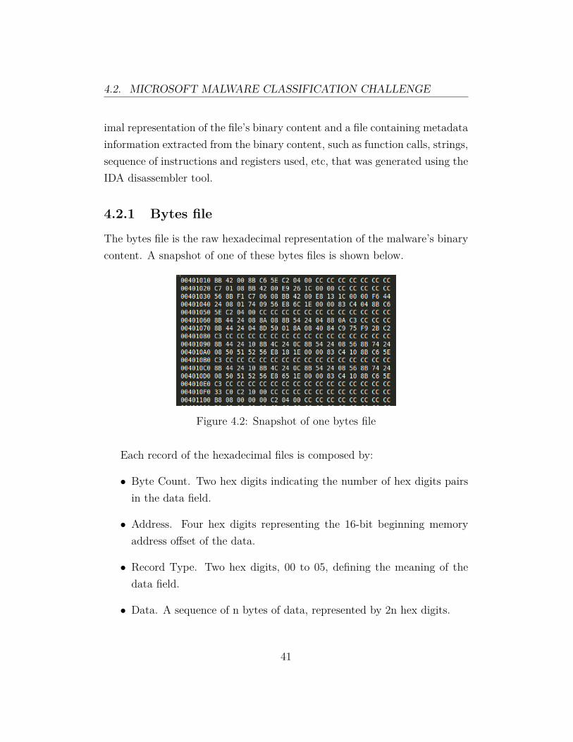
4.2.1 Bytes file
The bytes file is the raw hexadecimal representation of the malware’s binarycontent. A snapshot of one of these bytes files is shown below.
Figure 4.2: Snapshot of one bytes file
Each record of the hexadecimal files is composed by:
• Byte Count. Two hex digits indicating the number of hex digits pairsin the data field.
• Address. Four hex digits representing the 16-bit beginning memoryaddress offset of the data.
• Record Type. Two hex digits, 00 to 05, defining the meaning of thedata field.
• Data. A sequence of n bytes of data, represented by 2n hex digits.
41

4.2. MICROSOFT MALWARE CLASSIFICATION CHALLENGE
• Checksum. Two hex digits, a computed value that can be used to verifythe record has no errors.
4.2.2 ASM file
The asm file, generated by the disassembler tool, is a log containing vari-ous metadata such as rudimentary function calls, memory allocation, andvariable manipulation. A snapshot of one of these files is shown below.
Figure 4.3: Snapshot of one assembly code file
An assembly program is often divided into three sections:
1. The data section. It is used to declare initialized data or constants anddo not change at runtime.
2. The bss section. It is used for declaring variables. Contains uninitial-ized data.
3. The text section. It keeps the actual code of the program.
Apart from the previous sections, an assembly program can contain othersections such as:
• The rsrc section. It contains all the resources of the program.
• The rdata section. It holds the debug directory which stores the type,size and location of various types of debug information stored in thefile.
42

4.2. MICROSOFT MALWARE CLASSIFICATION CHALLENGE
• The idata section. It contains information about functions and datathat the program imports from DLLs.
• The edata section. It contains the list of the funcions and data thatthe PE file exports for other programs.
• The reloc section. It holds a table of base relocations. A base relocationis an adjustment to an instruction or initialized variable value that’sneeded if the loader couldn’t load the file where the linker assumed itwould.
Additionally, some other sections can appear as a result of applying a poly-morphic or metamorphic techniques to hide the actual code.
The assembly language consists of three types of statements:
1. Instructions or assembly language statements. Are used to tell theprocessor what to do. Instructions are entered one instruction per line.Each instruction has the following format:
[ l a b e l ] mnemonic [ operands ] [ ; comment ]
where the fields in brackets are optional. A basic instruction has twoparts: (1) the name of the instruction or the mnemonic to be executed(also known as opcodes); (2) the operands or the parameters of thecommand.
INC COUNT ; Increment the memory va r i ab l e COUNTMOV TOTAL, 48 ; Trans fe r the va lue 48 in the
; memory va r i ab l e TOTAL
Next you will find the top 10 most used x86 instructions in the trainingdataset.
43

4.2. MICROSOFT MALWARE CLASSIFICATION CHALLENGE
Figure 4.4: Top 10 opcodes in the training dataset
In addition, the average of instructions per each malware family is thefollowing.
Figure 4.5: Average of opcodes per malware family
44

4.2. MICROSOFT MALWARE CLASSIFICATION CHALLENGE
One particularity of the training dataset is that there are some mal-ware samples that due to code obfuscation techniques do not have anyinstruction.
#samplesRamnit 0Lollipop 2Kelihos_ver3 4Vundo 22Simda 0Tracur 0Kelihos_ver1 6Obfuscator.ACY 9Gatak 0
Table 4.1: Number of samples per class with 0 instructions
2. Assembler directives or pseudo-ops. Are commands part of the assem-bler syntax but are not related to the x86 processor instruction set. Allassembly directives start with a period (.).
. data
. bss
The .data and .bss directives change the current section to .data or.bss, respectively.
3. Macros. Are basically a text substitution mechanism. A macro is a se-quence of instructions, assigned by a name and could be used anywherein the program. The syntax for a macro definition is:
%macro macro_name number_of_params<macro body>%endmacro
45

4.3. WINNER’S SOLUTION
4.3 Winner’s solution
The competition was won by a team of three people, Jiwei Liu and XueerChen from the University of Pittsburgh and Xiaozhou Wang from RedmanTechnologies Inc. Their solution relied mainly in the extraction of the threefollowing features from malware.
1. Opcode 2,3 and 4-grams.
• They counted the frequent 1-gram opcodes by selecting only theopcodes that appear more than 200 times in at least one asm fileand they ended up with 165 features.
• All possible 2-gram counts were included (27225 features)
• The 3-gram and 4-gram counts which were greater than 100 in atleast one asm file were also included (21285 and 22384 features,respectively)
2. Segment line count. They counted the number of lines per section inthe asm file and they also counted the number of different sections in allmalware samples which curiously was 448 a number much greater than9, the number of sections in which an asm is usually divided. That’sbecause of the application of metamorphic and polymorphic techniques.
3. Asm file pixel intensity features. Instead of representing the bytes fileas pixels they read the asm file as a binary file. They found that thefirst 800 pixel intensities were very useful features.
Then, they used XGBoost(a machine learning library focused on gradientboosted trees) and cross-validation to find the subset of features that bestclassified the malware in classes and they finally obtained the lowest publicand private logloss of 0.003082695 and 0.002833228, respectively. In the nextfigure you can find the confusion matrix of the training data.
46

4.4. NOVEL FEATURE EXTRACTION, SELECTION AND FUSIONFOR EFFECTIVE MALWARE FAMILY CLASSIFICATION
Ramnit Lollipop Kelihos_ver3 Vundo Simda Tracur Kelihos_ver1 Obfuscator.ACY GatakRamnit 1541 0 0 0 0 0 0 0 0Lollipop 1 2476 0 0 0 1 0 0 0Kelihos_ver3 0 0 2942 0 0 0 0 0 0Vundo 0 0 0 475 0 0 0 0 0Simda 2 0 0 0 39 1 0 0 0Tracur 1 0 0 0 0 750 0 0 0Kelihos_ver1 0 0 0 0 0 0 398 0 0Obfuscator.ACY 0 0 1 0 0 0 0 1225 2Gatak 0 1 0 0 0 0 0 5 1007
Table 4.2: Winner’s solution: confusion matrix
where they classified correctly 10854 of 10868 samples (0, 9987%).
4.4 Novel Feature Extraction, Selection andFusion for Effective Malware Family Clas-sification
In [1] they presented an approach that extracts and combines different char-acteristics from malware and their fusion according to a perclass weightingparadigm. Their method achieved an accuracy of 0.998% on the MicrosoftMalware Challenge dataset but what is more interestingly about their ap-proach is that they also extracted feature patterns from images of malware.
Next you will find the different extracted set of features.
1. N-Gram (1G and 2G):1-Gram and 2-Gram features from the hexadecimal representation of bi-nary files described with a 256-dimensional vector and 2562-dimensionalvector for the 1-Gram and 2-Gram models, respectively.
2. Metadata (MD1 and MD2):They extracted the size of the file and the address of the first bytesequence.
47
4.4. NOVEL FEATURE EXTRACTION, SELECTION AND FUSIONFOR EFFECTIVE MALWARE FAMILY CLASSIFICATION
3. Entropy (ENT):Entropy can be defined as a measure of the amount of the disorder andit is used to detect the presence of obfuscation in malware files and forthis reason they computed the entropy of all the bytes in a malwarefile.
4. Image patterns (IMG1 and IMG2):They extracted the Haralick features and the Local Binary Patternsfeatures from each malware sample represented as a gray-scale image.
5. String length (STR):They extracted possible ASCII strings and its length from each PEusing its hex dump.
6. Symbol frequencies (SYM):The frequencies of the symbols -, +, *, ], [, ?, @ are extracted fromthe disassembled files because are typical of code designed to evadedetection by resorting to indirect calls or dynamic library loading.
7. Operation code (OPC):They counted the number of times a subset of 98 operation codes ap-peared in each disassembled file. These subset was selected based eitheron their commonness or on their frequent use in malicious applications.
8. Register (REG):They computed the frequency of use of the registers in x86 architecture.
9. Application Programming Interface (API):They measured the frequency of use of the top 794 frequent APIs usedin malware binaries based on the analysis performed in https://www.bnxnet.com/top-maliciously-used-apis/.
10. Section (SEC):They extracted different characteristics from sections in the disassem-
48
4.4. NOVEL FEATURE EXTRACTION, SELECTION AND FUSIONFOR EFFECTIVE MALWARE FAMILY CLASSIFICATION
bly files such as the total number of lines in .bss, .txt, .data, etc sectionsor the proportion of lines in each section compared to the whole file.
11. Data Define (DP):They computed the frequency of db, dw and dd instruction becausethere are malware samples that do not contain any API call and onlycontain few operation codes, because of packing.
12. Miscellaneous (MISC):This features are composed by the frequency of 95 keywords manuallychosen from the disassembled code.
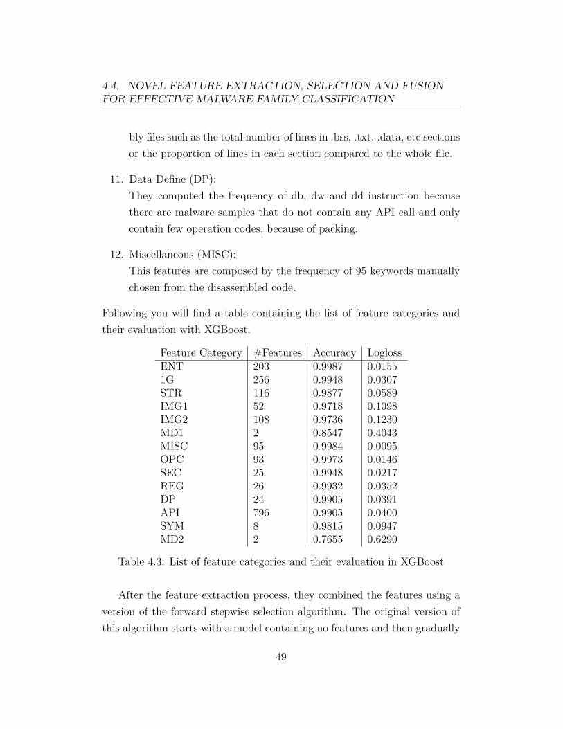
Following you will find a table containing the list of feature categories andtheir evaluation with XGBoost.
Feature Category #Features Accuracy LoglossENT 203 0.9987 0.01551G 256 0.9948 0.0307STR 116 0.9877 0.0589IMG1 52 0.9718 0.1098IMG2 108 0.9736 0.1230MD1 2 0.8547 0.4043MISC 95 0.9984 0.0095OPC 93 0.9973 0.0146SEC 25 0.9948 0.0217REG 26 0.9932 0.0352DP 24 0.9905 0.0391API 796 0.9905 0.0400SYM 8 0.9815 0.0947MD2 2 0.7655 0.6290
Table 4.3: List of feature categories and their evaluation in XGBoost
After the feature extraction process, they combined the features using aversion of the forward stepwise selection algorithm. The original version ofthis algorithm starts with a model containing no features and then gradually
49

4.4. NOVEL FEATURE EXTRACTION, SELECTION AND FUSIONFOR EFFECTIVE MALWARE FAMILY CLASSIFICATION
increases the feature set by adding one feature at each iteration. Insteadof considering one feature at a time, they added all the subset of featuresbelonging to a feature category at a time, until when adding more featuresdidn’t increase the value of logloss. By combining the feature categories asdescribed earlier, they achieved a test logloss of 0.0063 positioning its solutionamong the top 10 in the competition.
50

4.5. DEEP LEARNING FRAMEWORKS
4.5 Deep Learning Frameworks
Deep Learning is a hot field in Artificial Intelligence and Machine Learning,and thus, there are various deep learning libraries available open-source. Themost popular are:
1. Caffe.It is a python deep learning framework developed by the Berkeley Vi-sion and Learning Center. It allows you to define if train using theCPU or the GPU easily. Caffe benefits from having a huge repositorywith pre-trained neural network models suited for many problems. Ithas a great implementation for convolutional networks but it has noimplementation for recurrent networks.
2. Theano.It is a python deep learning library which make use of symbolic graphfor programming the networks. It also allows you to visualize the com-putation graphs with d3viz.
3. TensorFlow.It is written with a Python API over a C/C++ engine that makes itrun fast. It is more than a deep learning framework, and it has tools tosupport reinforcement learning and other algorithms. In addition, Ten-sorFlow can also be deployed in phones thanks that it can be compiledin ARM architectures.
4. Deeplearning4j.It is a deep learning framework developed in Java. It aims to be thescikit-learn library in the deep learning space.
5. Torch.It is a computational framework written in Lua that supports machinelearning algorithms. It has been used by large scale companies such as
51

4.5. DEEP LEARNING FRAMEWORKS
Google and Facebook. However, it is not as well-documented as otherdeep learning frameworks.
TensorFlow has been chosen mainly because it has a Python API, there’sa lot of documentation available and it has a large community that it con-tinuously develops the library. In addition, it is very easy to setup and tolearn and recently, they released TensorBoard, a tool to visualize TensorFlowgraphs and to plot some metrics such as the accuracy or the loss at each train-ing iteration. Moreover, it provides support for distributed computing sinceversion 0.8 (currently 0.11).
52

Chapter 5
Learning Feature Extractorsfrom Malware Images
The problem of malware detection and classification is a very complex taskand there’s no perfect approach to tackle it. For this reason AV vendors relyin hybrid approaches that make use of traditional signature-based, heuristic-based and machine learning methods as well as human analysis.
This chapter presents a novel approach for malware classification based onthe work performed by Nataraj et al. [21] which introduced the idea ofrepresenting malicious software as gray-scale images. Then, they extracteddifferent features using GIST and they used the k-nearest neighbor algorithmfor classification. Our approach differ in the point that we use ConvolutionalNeural Networks for learning discriminative patterns from the malware im-ages.
The next sections explain how malware can be visualized as images followedby the architectures of the different CNNs tested and its specifications aswell as the results obtained in the Kaggle’s competition.
53

5.1. VISUALIZING MALWARE AS GRAY-SCALE IMAGES
5.1 Visualizing malware as gray-scale images
This thesis is highly motivated by the work in [21] which is based on theobservation that images of different malware samples from the same familyappear to be similar while images of malware samples belonging to a differ-ent family are distinct. Moreover, if old malware is re-used to create newmalware binaries the resulting ones would be very similar visually.
In their work, they computed image based features to characterize malware.For that purpose, to compute texture features they used GIST [24]. Theresulting feature vectors were used to train a K-nearest neighbor classifierwith Euclidean distance. As introduced in [21], a given malware binary filecan be read as a vector of 8 bit unsigned integers and organized into a 2Darray. Then, this array can be visualized as a gray scale image in the range[0,255].
Figure 5.1: Visualizing Malware as a Gray-Scale Image
The main benefit of visualizing malware as an image is that the differentsections of a binary can be easily differentiated. In addition, as malware au-thors only change a small part of the code to produce new variants, imagesare useful to detect small changes while retain the global structure. In con-sequence, malware variants belonging to the same family appear to be verysimilar as images while also being distinct from images of other families.
54

5.1. VISUALIZING MALWARE AS GRAY-SCALE IMAGES
5.1.1 Malware families
Following are presented some malware files of each malware variant in thedataset. One particularity of the dataset is that the samples do not containthe PE header because it was removed to ensure sterility.
1. Ramnit. This type of malware is known to steal your sensitive infor-mation such as user names and passwords and it also can give accessto an illegitimate user to your computer.
Figure 5.2: Rammit samples
2. Lollipop. This malware shows ads in your browser and redirects yoursearch engine results. In addition, it tracks what you are doing on yourcomputer. This type of malware usually is downloaded from the pro-gram’s website or by some third-party software installation programs.
Figure 5.3: Lollipop samples
3. Kelihos_ver3. Third version of the Kelihos botnet. Kelihos is mainlyinvolved in spamming and theft of bitcoins. This trojan can give ac-cess and control of your computer to an illegitimate user and can alsocommunicate with other computers about sending spam emails, runmalicious programs and steal sensitive information.
55

5.1. VISUALIZING MALWARE AS GRAY-SCALE IMAGES
Figure 5.4: Kelihos_ver3 samples
4. Vundo. This trojan is known to cause popups and advertising for rogueantispyware programs. In addition, sometimes is used to perform denialof service attacks and also to deliver malware to other computers.
Figure 5.5: Vundo samples
5. Simda. It is a family of backdoors that try to steal sensitive informationsuch as usernames, passwords and certificates via its keylogging andHTML injection routines. It also can give a hacker access to yourcomputer.
Figure 5.6: Simda samples
6. Tracur. This trojan hijacks results from different search engines suchas google, youtube, yahoo, etc, and redirects to a different web page. Italso give a hacker access to your computer and can be used to downloadother types of malware.
56

5.1. VISUALIZING MALWARE AS GRAY-SCALE IMAGES
Figure 5.7: Tracur samples
7. Kelihos_ver1. First version of the Kelihos botnet. It was first discov-ered at the end of 2010 having infected 45.000 machines and sendingabout 4 billions spam messages per day.
Figure 5.8: Kelihos_ver1 samples
8. Obfuscator.ACY. This class comprises all malware that has been ob-fuscated to hide their purposes and to not be detected. The malwarethat lies underneath this obfuscation can have almost any purpose.
Figure 5.9: Obfuscator.DCY samples
9. Gatak. It is a trojan that gathers information about your pc and sendsit to a hacker. It also downloads other malware files in your computer.This trojan is usually downloaded when downloading a key generatoror a software crack.
57

5.1. VISUALIZING MALWARE AS GRAY-SCALE IMAGES
Figure 5.10: Gatak samples
58
5.2. CNN ARCHITECTURES
5.2 CNN Architectures
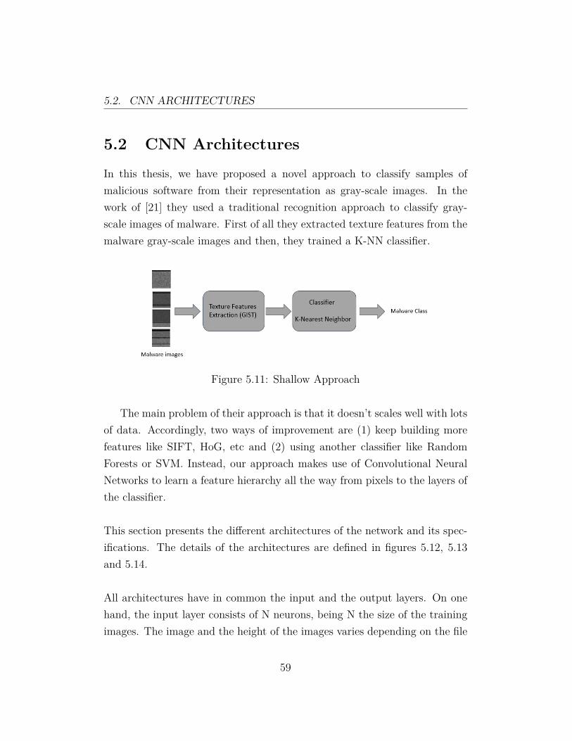
In this thesis, we have proposed a novel approach to classify samples ofmalicious software from their representation as gray-scale images. In thework of [21] they used a traditional recognition approach to classify gray-scale images of malware. First of all they extracted texture features from themalware gray-scale images and then, they trained a K-NN classifier.
Figure 5.11: Shallow Approach
The main problem of their approach is that it doesn’t scales well with lotsof data. Accordingly, two ways of improvement are (1) keep building morefeatures like SIFT, HoG, etc and (2) using another classifier like RandomForests or SVM. Instead, our approach makes use of Convolutional NeuralNetworks to learn a feature hierarchy all the way from pixels to the layers ofthe classifier.
This section presents the different architectures of the network and its spec-ifications. The details of the architectures are defined in figures 5.12, 5.13and 5.14.
All architectures have in common the input and the output layers. On onehand, the input layer consists of N neurons, being N the size of the trainingimages. The image and the height of the images varies depending on the file
59

5.2. CNN ARCHITECTURES
size and thus, before feeding the images as input all images had been down-sampled to 32 by 32 pixels. In consequence, N is equals to 32∗32 = 1024. Onthe other hand, all architectures have an output layer of 9 neurons becausethe architectures are designed to handle a 9-class classification problem. Inaddition, after each densely-connected layer it was applied dropout to reduceoverffiting.
To determine the parameters for each architecture it was performed a gridsearch. Specifically, the grid search was used to determine the optimum learn-ing rate, the size of the kernels of each convolutional layer and the numberof filters applied and also the number of neurons in each densely-connectedlayer. Finally, to reduce the search space some parameters were fixed such asthe mini-batch size to 256, the region of the max-pooling layer to 2x2 withstride equals to 2 and the learning rate to 0.001
60

5.2. CNN ARCHITECTURES
5.2.1 CNN A: 1C 1D
The architecture consists of:
1. Input layer of NxN pixels (N=32).
2. Convolutional layer (64 filter maps of size 11x11).
3. Max-pooling layer.
4. Densely-connected layer (4096 neurons)
5. Output layer. 9 neurons.
The input layer consists of 32x32 neurons and is followed by a convolutionallayer composed by 64 filters of size 11x11. The output of the convolutionallayer is (32−11+1)∗(32−11+1) = 22∗22 = 484 for each feature map. As aresult, the total output of the convolutional layer is 22∗22∗64 = 30976. Afterthat, the pooling layer takes the output of each feature map from the con-volutional layer and outputs the maximum activation of all 2x2 regions. Inconsequence, the output of the pooling layer is reduced to 11∗11∗64 = 7744.The pooling layer is then followed by a fully-connected layer with 4096 neu-rons and every neuron of this layer is also connected to each one of theneurons in the output layer.
The number of learnable parameters P of this network is:
P = 1024∗(11∗11∗64)+64+(11∗11∗64)∗4096+4096+4096∗9+9 = 39690313
where (11 ∗ 11 ∗ 64) + 64 are the shared weights for every feature map and64 is the total number of shared bias.
61

5.2. CNN ARCHITECTURES
Figure 5.12: Overview architecture A: 1C 1D
5.2.2 CNN B: 2C 1D
The architecture consists of:
1. Input layer of NxN pixels (N=32).
2. Convolutional layer (64 filter maps of size 3x3).
3. Max-pooling layer.
4. Convolutional layer (128 filter maps of size 3x3).
5. Max-pooling layer.
6. Densely-connected layer (512 neurons).
7. Output layer. 9 neurons.
As in the previous architecture, the input layer consists of 32x32 neurons andis followed by a convolutional layer composed by 64 filters of size 3x3. The
62

5.2. CNN ARCHITECTURES
output of the convolutional layer is (32− 3 + 1)∗ (32− 3 + 1) = 30∗ 30 = 900for each feature map and a total of 30 ∗ 30 ∗ 64 = 57600. Next it is applied amax-pooling layer which takes as input the output of the convolutional layerand outputs the maximum activation of all 2x2 regions reducing the outputto 15 ∗ 15 ∗ 64. Then, the pooling layer is followed by another convolutionallayer of 128 filters with 3x3 receptive fields. After the convolutional layerfollows another pooling layer that takes as input the output of the previousconvolutional layer that is 13*13*128 and reduces the output to 7*7*128.Finally, the polling layer is followed by a densely-connected layer with 512neurons.
The number of learnable parameters P of this network is:
P = 1024 ∗ (3 ∗ 3 ∗ 64) + 64 + (15 ∗ 15 ∗ 64) ∗ (3 ∗ 3 ∗ 128) + 128+
+(7 ∗ 7 ∗ 128) ∗ 512 + 512 + 512 ∗ 9 + 9 = 20395209
where (3 ∗ 3 ∗ 64) + 64 and (3 ∗ 3 ∗ 128) + 128 are the shared weights for everyfeature map and 64 and 128 are the number of shared bias in the first andsecond convolutional layers,respectively.
63
5.2. CNN ARCHITECTURES
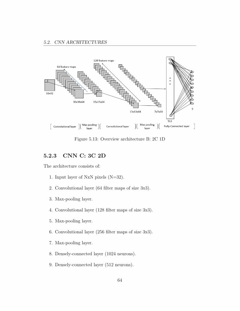
Figure 5.13: Overview architecture B: 2C 1D
5.2.3 CNN C: 3C 2D
The architecture consists of:
1. Input layer of NxN pixels (N=32).
2. Convolutional layer (64 filter maps of size 3x3).
3. Max-pooling layer.
4. Convolutional layer (128 filter maps of size 3x3).
5. Max-pooling layer.
6. Convolutional layer (256 filter maps of size 3x3).
7. Max-pooling layer.
8. Densely-connected layer (1024 neurons).
9. Densely-connected layer (512 neurons).
64

5.2. CNN ARCHITECTURES
10. Output layer. 9 neurons.
It starts with an input layer with 32x32 neurons which is then followed by aconvolutional layer with 64 filters of size 3x3. The output of the convolutionallayer is 30x30x64 and is used to feed the following max-pooling layer thatreduces its input to 15x15x64. Next follows the second convolutional layerwith 128 filters of size 3x3. After the convolutional layer it follows the secondpooling layer that takes as input the output of the second convolutional layer(13 ∗ 13 ∗ 128) and outputs 128 feature maps of size 7x7. Moreover, a thirdconvolutional layer with 256 filters of size 3x3 follows the second pooling layerwhich outputs 256 feature maps of size 5x5. Additionally, a third poolinglayer follows the convolutional layer reducing the input to 256 feature mapsof size 3x3. Lastly, follows two densely-connected layers of 1024 and 512neurons, respectively.
The number of learnable parameters P of this network is:
P = 1024∗(3∗3∗64)+64+(15∗15∗64)∗(3∗3∗128)+128+(7∗7∗128)∗(3∗3∗256)+
+256 + (3 ∗ 3 ∗ 256) ∗ 1024 + 1024 + 1024 ∗ 512 + 512 + 512 ∗ 9 + 9 = 34519497
where (3∗3∗64)+64, (3∗3∗128)+128 and (3∗3∗256)+256 are the sharedweights for every feature map and 64 and 128 are the number of shared biasof the first, second and third convolutional layers, respectively.
65

5.2. CNN ARCHITECTURES
Figure 5.14: Overview architecture C: 3C 2D
66

5.3. RESULTS
5.3 Results
The content of this section is structured as follows. First are presented theresults of the CNNs obtained during training and validation and then, arepresented the scores achieved in the competition.
5.3.1 Evaluation
The dataset provided by Kaggle for training was divided into two:
1. The training set of size (N −N/10) = 9781
2. The validation set of size M = N/10 = 1086
where N is the total size of the dataset, N = 10868 and M = 1086. Thevalidation set was used to search the parameters of the networks and to knowwhen to stop training. In particular, we stopped training the network if thevalidation loss increased in 10 iterations.
The next figure shows the accuracy and the cross-entropy achieved by themodels presented in 5.2 until they reached the 100th training iteration.
67

5.3. RESULTS
(a) Training & Validation accuracy (b) Training & Validation Cross-Entropy
Figure 5.15: Approach A: CNNs training results
It can be observed that the performance of the CNN with only one con-volutional layer performs poorly than the other nets. Next you will find theperformance of the networks on the training set at the 500th iteration.
• CNN 1C 1D. Accuracy: 0.9857 Cross-entropy: 0.0968
Rammit Lollipop Kelihos_ver3 Vundo Simda Tracur Kelihos_ver1 Obfuscator.ACY GatakRammit 1534 0 0 0 1 0 0 1 5Lollipop 0 2375 0 0 0 4 0 0 98Kelihos_ver3 0 1 2937 0 0 0 0 0 4Vundo 0 0 0 472 0 0 2 0 1Simda 0 0 0 1 41 0 0 0 0Tracur 2 0 0 2 0 737 0 4 10Kelihos_ver1 0 0 0 0 0 0 387 0 11Obfuscator.ACY 0 0 0 0 0 1 0 1219 8Gatak 0 0 0 0 0 2 0 0 1011
Table 5.1: CNN 1C 1D: confusion matrix
• CNN 2C 1D. Accuracy: 0.9976 Cross-entropy: 0.0231
68

5.3. RESULTS
Rammit Lollipop Kelihos_ver3 Vundo Simda Tracur Kelihos_ver1 Obfuscator.ACY GatakRammit 1539 0 0 0 0 0 0 1 1Lollipop 0 2471 0 0 0 1 0 0 5Kelihos_ver3 0 0 2938 0 0 0 4 0 0Vundo 0 0 0 474 0 0 0 0 1Simda 0 0 0 1 41 0 0 0 0Tracur 0 0 0 0 0 750 0 0 1Kelihos_ver1 0 0 0 0 0 0 394 0 4Obfuscator.ACY 0 1 0 0 0 2 2 1223 0Gatak 0 0 0 0 0 0 0 0 1013
Table 5.2: CNN 2C 1D: confusion matrix
• CNN 3C 2D. Accuracy: 0.9938 Cross-entropy: 0.0257
Rammit Lollipop Kelihos_ver3 Vundo Simda Tracur Kelihos_ver1 Obfuscator.ACY GatakRammit 1533 0 0 0 0 1 0 5 2Lollipop 0 2443 0 0 0 1 0 0 33Kelihos_ver3 0 0 2938 0 0 0 4 0 0Vundo 0 0 0 474 0 0 0 0 1Simda 0 2 0 0 39 0 0 1 0Tracur 0 0 0 0 0 747 1 0 3Kelihos_ver1 0 0 0 0 0 0 393 0 4Obfuscator.ACY 0 3 0 0 0 1 3 1211 3Gatak 0 0 0 0 0 0 0 0 1013
Table 5.3: CNN 3C 2D: confusion matrix
It can be observed that the convolutional neural networks with one and threeconvolutional layers had problems mainly while labeling samples from Ram-mit, Lollipop, Tracur, Kelihos_ver1 and Obfuscator.ACY and they ended upmisclassifying some samples as belonging to the Gatak malware’s family. Inparticular, the major number of misclassifications had been produced fromsamples of the Lollipop family, with 98 and 33 incorrect classifications fromthe convolutional net with one and three convolutional layers, respectively.Moreover, it can be seen that the training error of the convolutional networkwith two layers is lower than the other two because it greatly reduced thenumber of samples misclassified as Gatak and it achieved a training accuracyof 0.9978 very near to the one obtained by the winner’s solution (0.9987) anda loss of 0.0231 which is also lower the obtained in [1] using only the subset offeatures named IMG1 (Haralick features) and IMG2 (Local Binary Patternfeatures) as represented in 4.3 which is 0.9718 & 0.1098 and 0.9736 & 0.1230,
69

5.3. RESULTS
respectively.
5.3.2 Testing
Usually, Kaggle provides a test set without label in their competitions andthe Microsoft Malware Classification Challenge is not different. Therefore,to evaluate our models using the test set we have to submit a file withthe predicted probabilities for each class to Kaggle. These submissions areevaluated using the multi-class logarithmic loss. The logarithmic loss metricis defined as:
logloss = − 1N
N∑i=1
M∑j=1
yi,jlog(pi,j)
where N is the number of observations, M is the number of class labels,log is the natural logarithm, yi,j is 1 if the observation i is in class j and 0otherwise, and pi,j is the predicted probability that observation i is in classj.
This type of evaluation metric provides extreme punishment for being con-fident and wrong. That is, if the algorithm makes a single prediction thatan observation is definitely true (1) when it is actually false, it adds infinityto the error score making every other observation pointless. Hence, in theircompetitions, Kaggle bound the predictions away from extremes by usingthe following formula:
logloss = − 1N
N∑i=1
(yilog(pi) + (1− yi)log(1− pi))
Moreover, the submitted probabilities are not required to sum to one becausethey are rescaled prior to being scored.
Additionally, submissions in Kaggle are evaluated with two scores, the publicscore and the private score where the first one is calculated on approximately
70
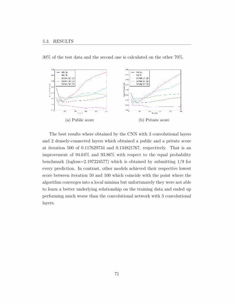
5.3. RESULTS
30% of the test data and the second one is calculated on the other 70%.
(a) Public score (b) Private score
The best results where obtained by the CNN with 3 convolutional layersand 2 densely-connected layers which obtained a public and a private scoreat iteration 500 of 0.117629734 and 0.134821767, respectively. That is animprovement of 94.64% and 93.86% with respect to the equal probabilitybenchmark (logloss=2.197224577) which is obtained by submitting 1/9 forevery prediction. In contrast, other models achieved their respective lowestscore between iteration 50 and 100 which coincide with the point where thealgorithm converges into a local minima but unfortunately they were not ableto learn a better underlying relationship on the training data and ended upperforming much worse than the convolutional network with 3 convolutionallayers.
71

Chapter 6
Convolutional Neural Networksfor Classification of MalwareDisassembly Files
As described in sections 4.3 and 4.4, the approaches that performed better inthe competition where those that extracted features from the disassembledfiles such as n-grams counts. A n-gram is a contiguous sequence of n itemsfrom a sentence. In our case, those items are opcodes extracted from thedisassembled files. However, the main problem that has extracting those n-grams is that the number of features extracted increases exponentially as Nincreases. In particular, a 2-gram model will result in a two-dimensional ma-trix of size 2562 = 65536, a 3-gram model will result in a three-dimensionalmatrix of 2563 = 16777216 features, a 4-gram model in a four-dimensionalmatrix of 2564 = 4294967296 and so on which turns out to be very compu-tationally expensive.
In this thesis, it is used the CNN architecture introduced by Yoon Kimin [12] as an alternative to n-grams because is much more computationallyefficient.
72
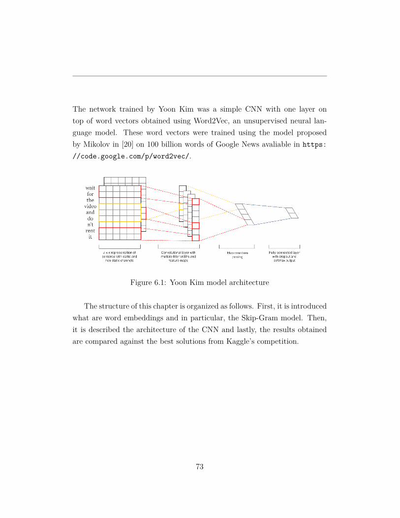
The network trained by Yoon Kim was a simple CNN with one layer ontop of word vectors obtained using Word2Vec, an unsupervised neural lan-guage model. These word vectors were trained using the model proposedby Mikolov in [20] on 100 billion words of Google News avaliable in https://code.google.com/p/word2vec/.
Figure 6.1: Yoon Kim model architecture
The structure of this chapter is organized as follows. First, it is introducedwhat are word embeddings and in particular, the Skip-Gram model. Then,it is described the architecture of the CNN and lastly, the results obtainedare compared against the best solutions from Kaggle’s competition.
73

6.1. REPRESENTING OPCODES AS WORD EMBEDDINGS
6.1 Representing Opcodes as Word Embed-dings
Traditionally, Natural Language Systems treated words as symbols, creatingencodings that are randomly generated and do not provide useful informa-tion for the system regarding the relationship among symbols. For example,"The" may be represented "Id156". By using vector representations of wordsthese problems are solved. There are various techniques of language model-ing that allow to map words or phrases from vocabulary, let’s say the Englishlanguage, to vectors of real numbers in a low-dimensional space. These set oflanguage models differ in the way they learn vector representation of wordsbut are all based on the distributional hypothesis which considers that wordsthat are used and occur in the same contexts tend to share semantic meaning.
The approaches that are based on this hypothesis can be divided broadlyinto two categories:
• Count-based methods. They compute how often some word co-occurswith its neighbors in a corpus and then they map these count-basedstatistics to a vector for each word.
• Predictive methods. They try to predict a word given its neighbors interms of learned small, dense embedding vectors.
Word2Vec [20] is a very efficient predictive model for learning word embed-dings. Word2Vec comes with two different approaches to learn the vectorrepresentations of words: (1) the Continuous Bag of Words (CBOW) and(2) the Skip-Gram model. The main difference between both models is thatCBOW predicts target words from source context words while the skip-grammodel predicts source context words from target words (the context of a wordare the words to the left of the target and the words to the right of the target).
74

6.1. REPRESENTING OPCODES AS WORD EMBEDDINGS
To learn the word embeddings we used the Skip-Gram approach and thus, anexplanation of the CBOW model is not provided because it is out of scope.
6.1.1 Skip-Gram model
The Skip-Gram model tries to predict each context word from its target word.Thus, the input to the model is wi and the output is wi−2,wi−1,wi+1,wi+2 ifa window size of 2 is used.
Figure 6.2: Skip-gram model architecture
As the network can’t be feed with words just as text strings is needed away to represent words. For that purpose, first it is build a vocabulary ofwords from the malware training samples. In the case all operation codesappear in the samples the vocabulary will consist of 665 words. Accordingly,a word like "push" is going to be represented as a one-hot vector. This vectorwill have 665 components (one for every word in the vocabulary) and in theposition corresponding to the word "push" it will place a 1 and 0s in all of
75

6.1. REPRESENTING OPCODES AS WORD EMBEDDINGS
the other positions.
The output layer depends on the window size. Thus, for a window sizeone (just predicting one word to the left and to the right of the targets word)the network will output a two-dimensional vector, with one dimension of thevector containing the probabilities of the words in the vocabulary to appearat the left of the target word and the other dimension containing the prob-abilities of the words in the vocabulary to appear at the right of the targetword. The dimension of the hidden layer or embedding layer corresponds toV ∗ E, where V is the size of the vocabulary and E is the embedding size.
The training objective of the Skip-gram model is to find word representationsthat are useful for predicting surrounding words in a corpora. Formally, givena sentence of words w1, w2, ..., wT the objective is to maximize the averagelog probability defined as:
1T
T∑t=1
∑−c≤j≤c,j 6=0
log p(wt+j|wt)
where c is the size of the training context (Larger c results in more trainingexamples and can lead to a higher accuracy at the expense of the trainingtime) and p(wo|wI) is formulated as:
p(wo|wI) = exp(vwoTvwI
)∑Ww=1 exp(vw
′TvwI)
where vw and vw′ are the "input" and "output" vector representations of words
in the vocabulary and W is the number of words in the vocabulary.
The main drawback of this formulation is that as W is often large (105)the cost of computing 5log p(wt+j|wt) is impractical. An alternative of thefull softmax is the Noise-Contrastive Estimation (NCE). NCE postulates
76
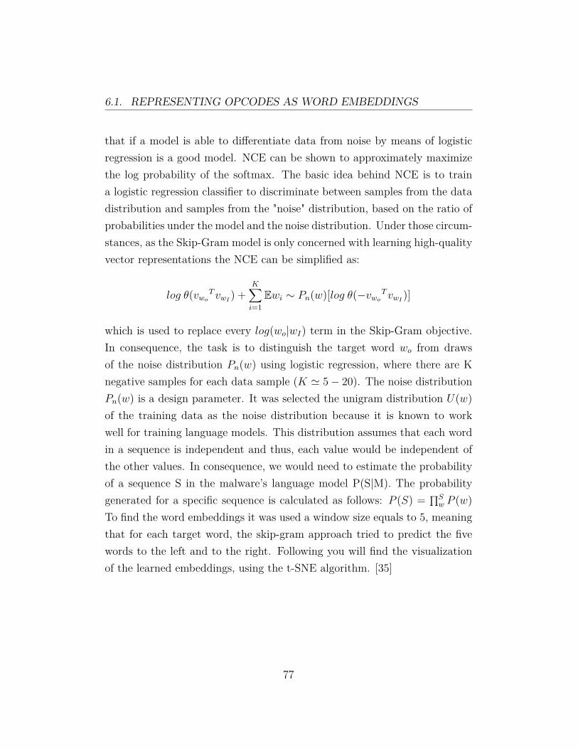
6.1. REPRESENTING OPCODES AS WORD EMBEDDINGS
that if a model is able to differentiate data from noise by means of logisticregression is a good model. NCE can be shown to approximately maximizethe log probability of the softmax. The basic idea behind NCE is to traina logistic regression classifier to discriminate between samples from the datadistribution and samples from the "noise" distribution, based on the ratio ofprobabilities under the model and the noise distribution. Under those circum-stances, as the Skip-Gram model is only concerned with learning high-qualityvector representations the NCE can be simplified as:
log θ(vwo
TvwI) +
K∑i=1
Ewi ∼ Pn(w)[log θ(−vwo
TvwI)]
which is used to replace every log(wo|wI) term in the Skip-Gram objective.In consequence, the task is to distinguish the target word wo from drawsof the noise distribution Pn(w) using logistic regression, where there are Knegative samples for each data sample (K ' 5− 20). The noise distributionPn(w) is a design parameter. It was selected the unigram distribution U(w)of the training data as the noise distribution because it is known to workwell for training language models. This distribution assumes that each wordin a sequence is independent and thus, each value would be independent ofthe other values. In consequence, we would need to estimate the probabilityof a sequence S in the malware’s language model P(S|M). The probabilitygenerated for a specific sequence is calculated as follows: P (S) = ∏S
w P (w)To find the word embeddings it was used a window size equals to 5, meaningthat for each target word, the skip-gram approach tried to predict the fivewords to the left and to the right. Following you will find the visualizationof the learned embeddings, using the t-SNE algorithm. [35]
77

6.1. REPRESENTING OPCODES AS WORD EMBEDDINGS
Figure 6.3: t-SNE representation of the word embeddings
For instance, the opcodes whose vector representations are most similarto the opcode "push" are:
1. pop
2. insertps
3. fucomp
which makes sense because tons of push instructions in malware files arefollowed by the pop instruction or viceversa and are the two opcodes mostused. To compute the similarity between two vectors p and q it was used theEuclidean distance.
d(p, q) = d(q, p) =√√√√ n∑
i=1(qi − pi)2
78

6.2. CONVOLUTIONAL NEURAL NETWORK ARCHITECTURE
6.2 Convolutional Neural Network Architec-ture
The input of the network is a window of N (default=10000) opcodes fromthe disassembly file represented as one-hot vectors of size V. As the numberof opcodes in every file is different we just extracted the first 10000 opcodesof each file. The criteria used to select N is the following:
• A lower N will result in not capturing enough information of malwaresamples belonging to the classes Ramnit and Lollipop which the averagenumber of instructions per sample is greater than 20000.
• A higher N will result in an increase in the time needed for trainingthe network.
• 10000 is greater than the average of opcodes of almost all malwaresamples except from those belonging to the Ramnit and Lollipop family(figure 4.5).
In addition, all malware files with less than N opcodes will be filled withUNKNOWN tokens ("UNK").
Regarding the embedding layer, is composed by a V x E matrix and it isthe responsible of mapping the opcodes into low-dimensional vector repre-sentations. It’s essentially a lookup table that can be learned during trainingor it can be initialized using the vector representations learned using anylanguage model such as the Skip-Gram approach explained in section 6.1.1.
79

6.2. CONVOLUTIONAL NEURAL NETWORK ARCHITECTURE
Figure 6.4: CNN Embedding layer output
The embedding layer is followed by a convolutional layer which have K(default 64) filters of different sizes (i x E, where i is an integer value rep-resenting the number of opcodes it covers. Each filter slides over the wholeembedded input, but varies in how many opcodes it covers.
80

6.2. CONVOLUTIONAL NEURAL NETWORK ARCHITECTURE
Figure 6.5: CNN Convolutional layer output
Following the convolutional layer it is performed max-pooling over theoutput of a specific filter size and leaves us with an output of size K, whichis essentially a feature vector. Then, the output of the max-pooling layeris combined into one long feature vector. Lastly, the features obtained inthe previous layer (with dropout applied) are used to generate the desiredpredictions by doing a matrix multiplication and selecting the class with thehighest score.
81

6.2. CONVOLUTIONAL NEURAL NETWORK ARCHITECTURE
Figure 6.6: CNN Max-pooling & output layer
82
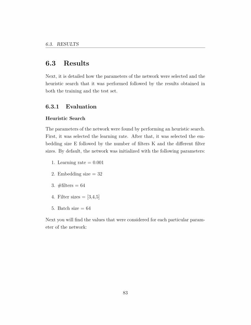
6.3. RESULTS
6.3 Results
Next, it is detailed how the parameters of the network were selected and theheuristic search that it was performed followed by the results obtained inboth the training and the test set.
6.3.1 Evaluation
Heuristic Search
The parameters of the network were found by performing an heuristic search.First, it was selected the learning rate. After that, it was selected the em-bedding size E followed by the number of filters K and the different filtersizes. By default, the network was initialized with the following parameters:
1. Learning rate = 0.001
2. Embedding size = 32
3. #filters = 64
4. Filter sizes = [3,4,5]
5. Batch size = 64
Next you will find the values that were considered for each particular param-eter of the network:
83

6.3. RESULTS
1. Learning rate: 0.01, 0.005, 0.001, 0.0005
(a) Accuracy Comparison (b) Cross-entropy Comparison
Figure 6.7: Heuristic Search: Learning Rate
It was selected a λ = 0.001 because a large learning rate can make thegradient descent to overstep the minimum and also it has been testedin scientific publications that the value chosen works really well.
2. Embedding size: 8, 16, 32, 64
(a) Accuracy Comparison (b) Cross-entropy Comparison
Figure 6.8: Heuristic Search: Embedding size
It can be observed in the plot that both the CNN trained with E=32
84
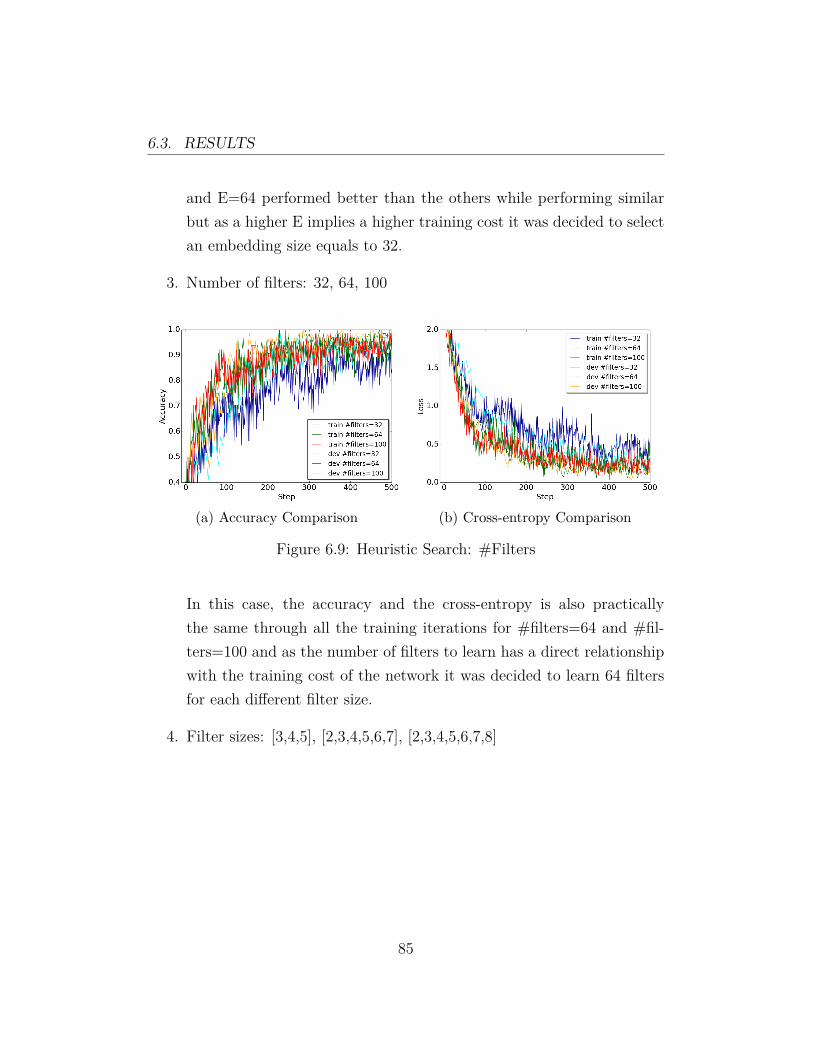
6.3. RESULTS
and E=64 performed better than the others while performing similarbut as a higher E implies a higher training cost it was decided to selectan embedding size equals to 32.
3. Number of filters: 32, 64, 100
(a) Accuracy Comparison (b) Cross-entropy Comparison
Figure 6.9: Heuristic Search: #Filters
In this case, the accuracy and the cross-entropy is also practicallythe same through all the training iterations for #filters=64 and #fil-ters=100 and as the number of filters to learn has a direct relationshipwith the training cost of the network it was decided to learn 64 filtersfor each different filter size.
4. Filter sizes: [3,4,5], [2,3,4,5,6,7], [2,3,4,5,6,7,8]
85
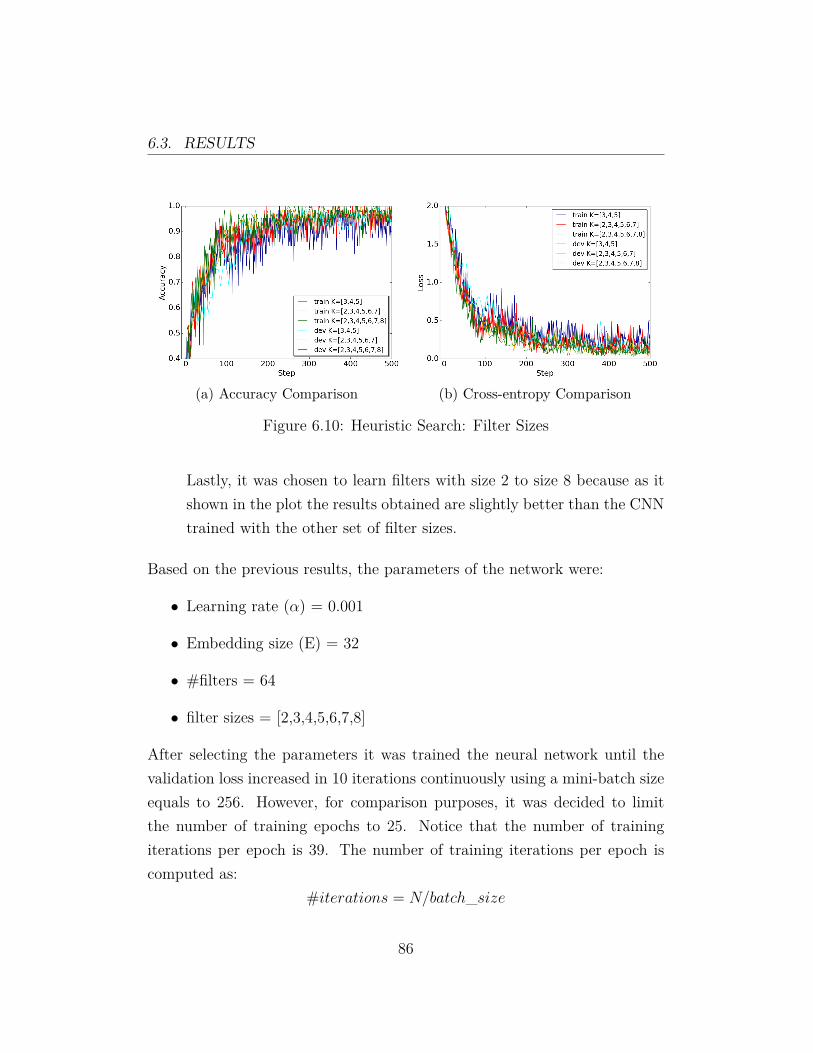
6.3. RESULTS
(a) Accuracy Comparison (b) Cross-entropy Comparison
Figure 6.10: Heuristic Search: Filter Sizes
Lastly, it was chosen to learn filters with size 2 to size 8 because as itshown in the plot the results obtained are slightly better than the CNNtrained with the other set of filter sizes.
Based on the previous results, the parameters of the network were:
• Learning rate (α) = 0.001
• Embedding size (E) = 32
• #filters = 64
• filter sizes = [2,3,4,5,6,7,8]
After selecting the parameters it was trained the neural network until thevalidation loss increased in 10 iterations continuously using a mini-batch sizeequals to 256. However, for comparison purposes, it was decided to limitthe number of training epochs to 25. Notice that the number of trainingiterations per epoch is 39. The number of training iterations per epoch iscomputed as:
#iterations = N/batch_size
86

6.3. RESULTS
where N is the total size of the training dataset (N=9781). Next you willfind their respective confusion matrices and also the accuracy and the cross-entropy of the models until epoch 25.
(a) Training & Validation Accuracy (b) Training & Validation Cross-Entropy
Figure 6.11: Approach B: CNNs training results
• CNN without pretrained word embeddings. Accuracy: 0.9952 Cross-Entropy: 0.0203
Ramnit Lollipop Kelihos_ver3 Vundo Simda Tracur Kelihos_ver1 Obfuscator.ACY GatakRamnit 1537 0 0 0 0 0 0 4 0Lollipop 4 2471 0 2 0 0 0 1 0Kelihos_ver3 0 0 2938 4 0 0 0 0 0Vundo 0 0 0 474 0 0 0 1 0Simda 0 0 0 0 42 2 0 0 1Tracur 3 0 0 1 0 744 0 3 0Kelihos_ver1 0 0 0 6 0 0 392 0 0Obfuscator.ACY 11 0 0 9 0 0 0 1208 0Gatak 0 0 0 0 0 0 0 3 1010
Table 6.1: CNN without pretrained word embeddings: confusion matrix
• CNN with pretrained word embeddings. Accuracy: 0.9947 Cross-Entropy:0.0243
87
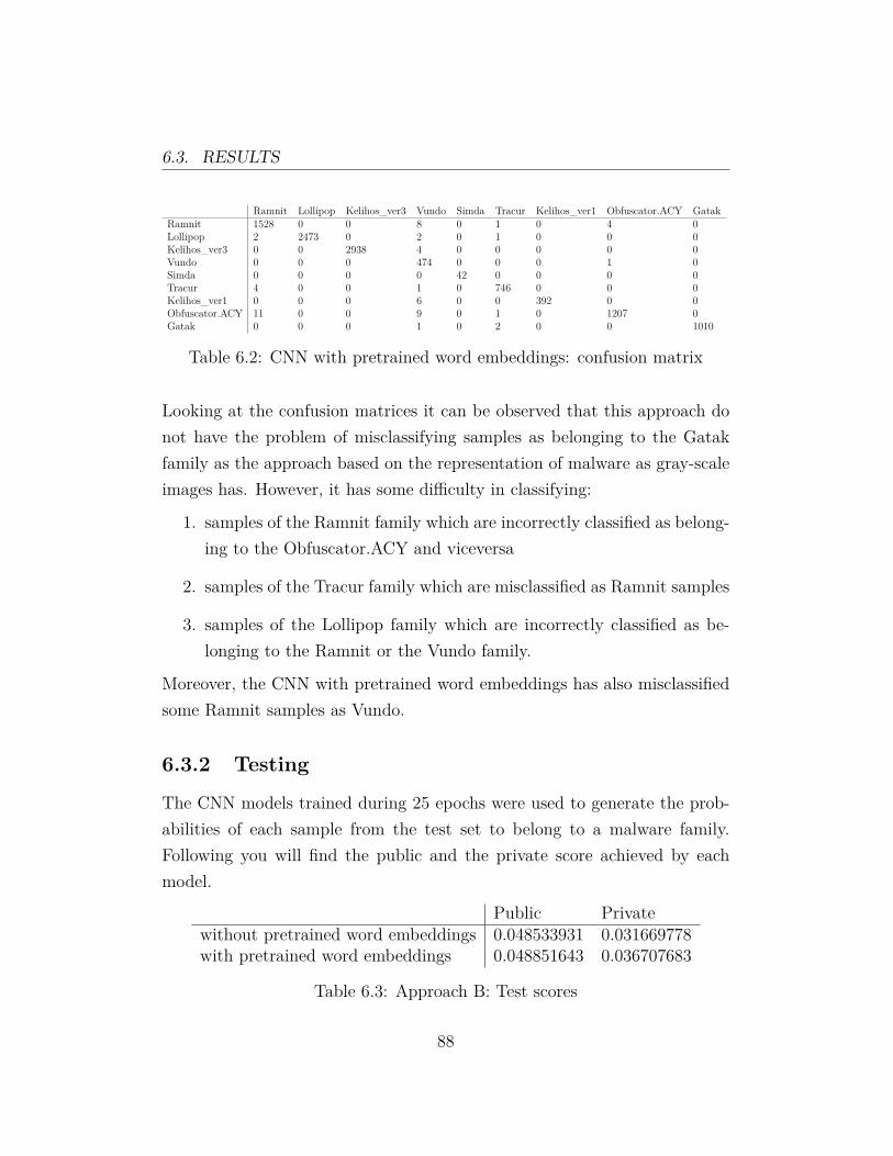
6.3. RESULTS
Ramnit Lollipop Kelihos_ver3 Vundo Simda Tracur Kelihos_ver1 Obfuscator.ACY GatakRamnit 1528 0 0 8 0 1 0 4 0Lollipop 2 2473 0 2 0 1 0 0 0Kelihos_ver3 0 0 2938 4 0 0 0 0 0Vundo 0 0 0 474 0 0 0 1 0Simda 0 0 0 0 42 0 0 0 0Tracur 4 0 0 1 0 746 0 0 0Kelihos_ver1 0 0 0 6 0 0 392 0 0Obfuscator.ACY 11 0 0 9 0 1 0 1207 0Gatak 0 0 0 1 0 2 0 0 1010
Table 6.2: CNN with pretrained word embeddings: confusion matrix
Looking at the confusion matrices it can be observed that this approach donot have the problem of misclassifying samples as belonging to the Gatakfamily as the approach based on the representation of malware as gray-scaleimages has. However, it has some difficulty in classifying:
1. samples of the Ramnit family which are incorrectly classified as belong-ing to the Obfuscator.ACY and viceversa
2. samples of the Tracur family which are misclassified as Ramnit samples
3. samples of the Lollipop family which are incorrectly classified as be-longing to the Ramnit or the Vundo family.
Moreover, the CNN with pretrained word embeddings has also misclassifiedsome Ramnit samples as Vundo.
6.3.2 Testing
The CNN models trained during 25 epochs were used to generate the prob-abilities of each sample from the test set to belong to a malware family.Following you will find the public and the private score achieved by eachmodel.
Public Privatewithout pretrained word embeddings 0.048533931 0.031669778with pretrained word embeddings 0.048851643 0.036707683
Table 6.3: Approach B: Test scores
88

6.3. RESULTS
The CNN without pretrained word embeddings achieved an improvementof 98,56% with respect to the equal probability benchmark while the CNNwith pretrained word embeddings achieved an improvement of 98,33%. Bothmodels are very close in terms of performance and no one can be declaredas better than the other. May the fact of generating the vectors represen-tentations of words using samples of malware instead of using goodware isthe cause of this situation. Probably if the input of the Skip-Gram modelused to learn the word embeddings had been samples of goodware the resultswould have been quite different. That’s because instructions such as xor ornop are commonly used by malware author’s for obfuscation purposes. Onone hand the exclusive OR (XOR) operation is commonly used to obfuscateparticular sensitive strings in the code such as URLs or registry keys. Thistype of obfuscation works like this:
1. The attacker chooses a 1-byte value to act as a key (range 0 -255).
2. Then malware’s code iterates through every byte of the data that needsto be encoded, XOR’ing each byte with the selected key.
When the attacker needs to deobfuscate the string, it repeats the step #2XOR’ing each byte in the encoded string with the key value.
On the other hand, the No operation (NOP) is used in a technique calleddead-code insertion which simply adds some ineffective and redundant in-structions to change the appearance of code while keeping its behavior intact.
From my point of view, I think that a better representation of the wordsin the vocabulary would have been achieved if goodware had been used asthe training data because the previous mentioned techniques and lots morenot explained in this thesis might produce unnecessary noise in the embed-dings.
89

Chapter 7
Conclusions
This master thesis studies the problem of classifying malware into their corre-sponding families. In order to explore the problem, we used one of the mostrecent and biggest datasets publicly available which was provided by Mi-crosoft for the BigData Innovators Gathering Cup (BIG 2015). This datasetprovides two files for each malware sample.
1. The hexadecimal representation of the file’s binary content.
2. The disassembled file generated by the IDA (Interactive DisAssembler)tool which contains various metadata information extracted from thebinary content. Metadata information contains instructions and regis-ters used by the malware, as well as the functions and data importedfrom DLLs.
This thesis presents two novel and scalable approaches using ConvolutionalNeural Networks to recognize the family a malware sample belongs.
• The first approach is motivated by [21] which introduced the idea ofrepresenting the malware’s binary content as gray-scale images. Themain benefit of visualizing malware as an image is that the differentsections of the binary can be easily differentiated. Their work is based
90

on the observation that images of different malware samples from thesame family appear to be similar while images of malware samplesbelonging to a different family are distinct. This property is useful toclassify new malware binaries that have been created by re-using oldmalware. That’s because images are useful to detect small changeswhile retaining the global structure and the new samples would bevery similar visually to the old ones. In consequence, in this thesis,we studied the application of CNNs to learn a feature hierarchy all theway from pixels to the layers of the classifier.
• The second approach uses the architecture introduced by Yoon Kim in[12] for sentence classification but applied to a distinct domain. Insteadof classifying sentences from the English language we used their archi-tecture to classify malware samples using the x86 instructions extractedfrom the disassembled files. We trained two models, the first one with-out pretrained word embeddings and the second one with pretrainedword embeddings generated using the Skip-Gram model.
The first and the second approach obtained a score of 0.134821767 and0.031669778, respectively. That is an improvement of 93.86% and 98,56%with respect to the equal probability benchmark (logloss=2.1972245577) whichis obtained by submitting 1/9 for every prediction. Unfortunately, neitherapproach outperformed the winner’s solution of the competition which ob-tained a logloss equal to 0.002833228. That’s because their solution combineddifferent features such as opcode 2,3 and 4-grams as well as the number oflines per section in the disassembled files, among others. However, the re-sults obtained are quite promising because both approaches are able to clas-sify malware samples much faster than all those solutions that rely on themanually extraction of features and thus, are more scalable.
91

7.1. FUTURE WORK
7.1 Future Work
Even that both approaches have been successfully applied, there is still ahuge margin of improvement. From now on, consider that the CNN used toclassify malware based on their representation as gray-scale images is namedCNN A and the CNN used to classify malware given the x86 instructionsof the disassembled file is named CNN B. Hence, one way to improve theresults is by merging the output of the last fully-connected layer of CNN Aand the output of the max-pooling layer of CNN B. Notice that the resultingCNN should be feed with two types of data: (1) the pixels extracted from therepresentation of malware as gray-scale images and (2) the opcodes extractedfrom the disassembled files. The idea is somehow similar to how pretrainedword embeddings were load and used in the CNN trained on opcodes. First,both models are trained independently. Therefore, CNN A will learn low-level and high-level features from the images while CNN B will learn a setof features (opcode patterns) from the disassembled files. Then, the learnedfilters are loaded into the CNN that will combine both approaches and thenetwork is trained again to learn the weight matrix of the output layer. Themain advantage of combining both CNNs is that the resulting CNN might beable to solve the problems of each particular approach. In other words, themodel may not has problems while classifying Ramnit samples as belongingto the Gatak family and neither discriminating between the Obfuscator.ACYand the Ramnit families.
Additionally, there is still a lot of work to be done regarding the approachpresented in section 6. One possible modification would be to increase thenumber of input opcodes allowed from 10.000 to the maximum number ofopcodes in a file found in the entire dataset. By making this small modi-fication, all the information about every malware sample will be captured.In particular, this modification can help to improve the classification rate of
92

7.1. FUTURE WORK
samples belonging to the Ramnit and the Lollipop families. That’s becausesamples from both families contain more than 20.000 opcodes per file in av-erage.
Another possible modification is to expand the vocabulary by including theregisters, the data directives and the most common imported DLL functionsand API calls found in malware. That would be effective for classifying allthose samples that, because of applying code obfuscation techniques, do nothave any instruction. In contrast, by expanding the vocabulary, the numberof parameters to learn will increase, as well as the time needed for trainingthe CNN.
Finally, the word embeddings could be improved by using as training datasamples of executables belonging to goodware. The main idea is that thereare some of the disassembled files that have been obfuscated by applyingdifferent techniques such as using the dead-code insertion technique or theXOR operation, among others. In consequence, the word embeddings maynot be accurate enough and might not represent correctly the words in thevocabulary.
93

Bibliography
[1] Mansour Ahmadi, Dmitry Ulyanov, Stanislav Semenov, Mikhail Trofi-mov, and Giorgio Giacinto. Novel feature extraction, selection and fu-sion for effective malware family classification. In Proceedings of theSixth ACM Conference on Data and Application Security and Privacy,CODASPY ’16, pages 183–194, New York, NY, USA, 2016. ACM.
[2] Clint Feher Shlomi Dolev Asaf Shabtai, Robert Moskovitch and YuvalElovici. Detecting unknown malicious code by applying classificationtechniques on opcode patterns. In Security Informatics. 2012.
[3] Daniel Billar. Opcodes as predictor for malware. International Journalof Electronic Security and Digital Forensics, 1:156–168, 2007.
[4] R Manoharan Chandrasekar Ravi. Malware detection using windowsapi sequence and machine learning. International Journal of ComputerApplications, 43, 2012.
[5] John Duchi, Elad Hazan, and Yoram Singer. Adaptive subgradientmethods for online learning and stochastic optimization. J. Mach. Learn.Res., 12:2121–2159, July 2011.
[6] Ekta Gandotra, Divya Bansal, and Sanjeev Sofat. Malware analysis andclassification: A survey. Journal of Information Security, pages 56–64,2014.
94

BIBLIOGRAPHY
[7] Dragos Gavrilut, Mihai Cimpoes, Dan Anton, and Liviu Ciortuz. Mal-ware detection using machine learning. Proceedings of the InternationalMulticonference on Computer Science and Information Technology, page735–741, 2009.
[8] Li Deng George E. Dahl, Jack W. Stokes and Dong Yu. Large-scalemalware classification using random projections and neural network.ICASSP, 2013.
[9] Geoffrey E. Hinton. Rectified linear units improve restricted boltzmannmachines vinod nair. In Proceedings of the 27th International Conferenceon Machine Learning (ICML),, pages 807 – 814, 2010.
[10] S. Hochreiter. Untersuchungen zu dynamischen neuronalen netzen.diploma thesis, institut fur informatik, lehrstuhl prof. brauer, technischeuniversitat munchen, 1991.
[11] Javier Nieves Yoseba K. Penya Borja Sanz Igor Santos, Felix Brezoand Carlos Laorden. Opcode-sequence-based malware detection. InEngineering Secure Software and Systems, volume 5965.
[12] Yoon Kim. Convolutional neural networks for sentence classification.CoRR, abs/1408.5882, 2014.
[13] Diederik P. Kingma and Jimmy Ba. Adam: A method for stochasticoptimization. CoRR, abs/1412.6980, 2014.
[14] J.Z. Kolter and M.A. Maloof. Learning to detect and classify maliciousexecutables in the wild. Journal of Machine Learning Research, page2721–2744, 2006.
[15] Deguang Kong and Guanhua Yan. Discriminant malware distancelearning on structural information for automated malware classification.Technical report, SIGMETRICS’13, 2013.
95

BIBLIOGRAPHY
[16] Alex Krizhevsky, Ilya Sutskever, and Geoffrey E. Hinton. Imagenetclassification with deep convolutional neural networks. In Advances inNeural Information Processing Systems, 2012.
[17] Mu Li, Tong Zhang, Yuqiang Chen, and Alexander J. Smola. Efficientmini-batch training for stochastic optimization. In Proceedings of the20th ACM SIGKDD International Conference on Knowledge Discoveryand Data Mining, KDD ’14, pages 661–670, New York, NY, USA, 2014.ACM.
[18] Robert Lyda and James Hamrock. Using entropy analysis to find en-crypted and packed malware. IEEE Security and Analysis, 5:40–45,2007.
[19] Zahra Salehi Mahboobe Ghiasi, Ashkan Sami. Dynamic malware detec-tion using registers values set analysis.
[20] Tomas Mikolov, Ilya Sutskever, Kai Chen, Greg S Corrado, and JeffDean. Distributed representations of words and phrases and their com-positionality. In C. J. C. Burges, L. Bottou, M. Welling, Z. Ghahramani,and K. Q. Weinberger, editors, Advances in Neural Information Process-ing Systems 26, pages 3111–3119. Curran Associates, Inc., 2013.
[21] L. Nataraj, S. Karthikeyan, G. Jacob, and B. S. Manjunath. Malwareimages: Visualization and automatic classification, 2011.
[22] Anil Thomas Nikos Karampatziakis, Jack Stokes and Mady Marinescu.Using file relationships in malware classification. Detection of Intrusionsand Malware, and Vulnerability Assessment, 7591:1–20, 2013.
[23] Aude Oliva and Antonio Torralba. Modeling the shape of the scene: Aholistic representation of the spatial envelope. International Journal ofComputer Vision, 42:145–175, 2001.
96

BIBLIOGRAPHY
[24] Aude Oliva and Antonio Torralba. Modeling the shape of the scene: Aholistic representation of the spatial envelope. Int. J. Comput. Vision,42(3):145–175, May 2001.
[25] Ning Qian. On the momentum term in gradient descent learning algo-rithms. Neural Netw., 12(1):145–151, January 1999.
[26] Smita Ranvee and Swapnaja Hiray. Comparative analysis of feature ex-traction methods of malware detection. International Journal of Com-puter Applications, 120, 2015.
[27] Clint Feher Nir Nissim Robert Moskovitch, Dima Stopel and YuvalElovici. Unknown malcode detection via text categorization and theimbalance problem. IEEE International Conference on Intelligence andSecurity Informatics, pages 156–161, 2008.
[28] Joshua Saxe and Konstantin Berlin. Deep neural network based malwaredetection using two dimensional binary program features, 2015.
[29] Sjsu Scholarworks and Donabelle Bays. Structural entropy and meta-morphic malware, 2013.
[30] R. Sekar, M. Bendre, D. Dhurjati, and P. Bollineni. A fast automaton-based method for detecting anomalous program behaviors. In Proceed-ings of the 2001 IEEE Symposium on Security and Privacy, SP ’01,pages 144–, Washington, DC, USA, 2001. IEEE Computer Society.
[31] Ohm Sornil and Chatchai Liangboonprakong. Malware classificationusing n-grams sequential pattern feature. International Journal of In-formation Processing and Management, 4, 2013.
[32] Nitish Srivastava, Geoffrey Hinton, Alex Krizhevsky, Ilya Sutskever, andRuslan Salakhutdinov. Dropout: A simple way to prevent neural net-works from overfitting. J. Mach. Learn. Res., 15(1):1929–1958, January2014.
97

BIBLIOGRAPHY
[33] Kephart J.O. Tesauro, G.J. and Gregory B Sorkin. Neural networks forcomputer virus recognition. IEEE International Conference on Intelli-gence and Security Informatics, 11, 1996.
[34] Antonio Torralba, Kevin P. Murphy, William T. Freeman, and MarkRubin. Context-based vision system for place and object recognition.pages 273–280, 2003.
[35] L.J.P. van der Maaten and G.E. Hinton. Visualizing high-dimensionaldata using t-sne. 2008.
[36] Nitin Rai Veeramani R. Windows api based malware detection andframework analysis. International Journal of Scientific & EngineeringResearch, 3, 2012.
[37] Yanfang Ye, Lifei Chen, Dingding Wang, Tao Li, Qingshan Jiang, andMin Zhao. Sbmds: an interpretable string based malware detectionsystem using svm ensemble with bagging, 2009.
98


![arXiv:2005.13044v1 [cs.CV] 26 May 2020 · The advent of recurrent neural networks for handwriting recognition marked an important milestone reaching im- ... The alphabet defining](https://static.fdocuments.ec/doc/165x107/6054a65ef4b14c04b54c5d19/arxiv200513044v1-cscv-26-may-2020-the-advent-of-recurrent-neural-networks-for.jpg)