Contacto · PDF file4 Los Hidratos de Metano: un recurso cada vez más cercano 6 Luis...

Contacto SPES U M A R I O

Director: Oscar Secco • Editor: Luciano Fucello • Comité de Redacción: Hugo Carranza, Miguel A. Laffitte y Alejandro Luppi

Publicación de la SPE de Argentina Asociación Civil

Número 42, Mayo 2013

Contacto SPE Mayo 2013

1 Carta del Director

2 Un joven argentino en el

World Gas Conference,

Kuala Lumpur 2012

4 Los Hidratos de Metano:

un recurso cada vez más

cercano

6 Luis Rey y Pluspetrol:

una historia argentina

12 Gas Pipeline Simulation,

fundamentals and state of art

16 Comisión de Jóvenes

Profesionales:

Almuerzos petroleros

17 Capítulos Estudiantiles:

Resumen Actividades

Contacto SPE propiedad de la SPE de Argentina Asociación Civil

Los artículos y sus contenidos así como las opiniones publicadas en la presente Revista son de exclusiva responsabilidad de sus respectivos autores. Envíenos sus comentarios: [email protected]

Carta del DirectorPor oscar secco • [email protected]

En la etapa fundacional, previa a la for-mación de la Sociedad Civil en el 1992, varias presidencias se extendieron a más de un año. Así resulta que Alberto Gil ac-cede a la presidencia #29 de la Society of Petroleum Engineers de Argentina hecho que cubriremos en el próximo número.

En esta edición dedicamos buena parte de su contenido a las actividades de los Capítulos Estudiantiles y de los Jóvenes Profesionales, ambos grupos objeto de un interés tan tradicional como especial de la SPE. Entre ellas encontrarán la nota de Mauro Palavecino sobre su destacada par-ticipación en la ultima World Gas Conferen-ce en Kuala Lumpur, Malasia, hace un año.

Hemos reseñado la historia de la com-pañía Pluspetrol y de su creador, Luis Rey, un caso muy exitoso de protagonismo en el negocio petrolero en la Argentina.

El tema “Gas Pipeline Simulation” lo encontrarán en inglés, tal como fue pre-sentado en el pasado mes de Octubre por el profesor Andrzej Osiadacz: preten-demos que nuestra publicación sea cada vez mas bilingüe.

Y finalmente el articulo sobre los Hidra-tos de Metano, recurso hidrocarburífero que pareciera superar, a nivel mundial, al de las hoy míticas Shales. Una vez más se extiende el horizonte de los combus-tibles fósiles: el tan temido “pico” está cada vez mas lejano.

Como actores protagónicos del sector, los ingenieros estamos preparados para continuar asistiendo con nuestros cono-cimientos al esfuerzo de producción de

gas y petróleo requerido para eliminar las importaciones de gas y petróleo.

Nuestro vecino Brasil acaba de anun-ciar, luego de una pausa de reflexión de 5 años, los resultados de una licitación de nuevas áreas : la adjudicación de 142 bloques en el mar y en tierra a 30 Com-pañías, 12 de ellas brasileras; las que pa-garon 1400 millones de dólares por de-rechos de exploración. Simultáneamente Petrobras ha emitido deuda por valor de 11000 millones de dólares al 4% de inte-rés para su propio desarrollo. Deseamos que la suerte los siga acompañando, tan-to con la geología como con precios fir-mes del petróleo.

Como en otras ocasiones quienes fati-gamos en esta publicación solicitamos la opinión de los lectores: Si bien invitamos a que nos contacten sin limitaciones, en esta ocasión les pedimos muy especial-mente que cuando reciban en su domicilio u oficina este ejemplar nos avisen por mail ([email protected] ) de la fecha de su llegada. Agradecemos desde ya esta colaboración necesaria para mejorar el eslabón mas dé-bil de CONTACTO: su distribución. Además informamos que este número se atrasó 1 mes, lo compensaremos adelantando el próximo para fines de Agosto.

Finalmente quiero reconocer la impor-tante ayuda de Luciano Fucello en la pre-paración de este número, como también a la de la Dra. Magali Giovanelli Petito en la reseña de la historia de Pluspetrol y de su fundador.

Hasta el #43, con Salud y Confianza.

Foto por: Marcelo

Hirschfeldt

En este mes de Mayo se renovó la Comisión Directiva del SPEA, rito que no se ha de-jado de cumplir desde su fundación en el año 1977. Desde entonces 23 Socios fueron honrados con esta responsabilidad, 6 de ellos fueron reelectos.


Un joven argentino en el World Gas Conference, Kuala Lumpur, 2012

el comité de selección de Malasia, que eligió a los 7 ganadores.

La Youth Roundtable fue compuesta de la siguiente manera:

Representantes jóvenes:

1. Abhijeet Kulkarni (India)

2. Ivan Pyvovarenko (Australia)

3. Kristin Xueqin Wu (Holanda)

4. Maria Kraynova (Rusia)

5. Mauro Palavecino (Argentina)

6. Milton Takada (Brasil)

7. Shu Wu (China)

Representantes Sr.:

1. Juniwati Rahmat Husin (VP Human Rosources, Petronas)

2. Brian Buckley (CEO, Oman LNG)

3. Antonio Llarden (CEO, Enagas SA)

4. Emma Cochrane (VP, ExxonMobil Gas & Power Marketing Co.)

5. Hinda Gharbi (President, SLB Asia Pacific)

6. Anuar Taib (Country Chairman, Shell Malaysia)

La Conferencia Mundial de Gas es uno de los eventos más importantes a nivel mundial de la Industria del petróleo y el gas, organizada cada tres años por el IGU. La última edición, número 25, se realizó en Kuala Lumpur entre el 4 y el 8 de junio de 2012 (www.wgc2012.com), bajo el lema “Gas: sustentando el futuro crecimiento mundial”. La Conferencia al-bergó casi 5000 Delegados, representan-tes de las más reconocidas Empresas a nivel mundial, entre ellos 20 argentinos. La edición previa del WGC tuvo lugar en 2009 en Buenos Aires.

El Youth Programme del 25th WGC integró diversas actividades organizadas especialmente para los jóvenes, como charlas de Profesionales Senior de la In-dustria del Petróleo y el Gas, debates de Líderes de la Industria, y la actividad más destacable del Youth Programme: la Youth Roundtable.

El Programa de Jóvenes del WGC se organizó con un tema eje cada día, de la siguiente manera:

Martes 5 de Junio: ‘Think About Gas’ Miércoles 6 de Junio: ‘Talk About Gas’ Jueves 7 de Junio: ‘To Appreciate Gas’

En total durante los tres días del Youth Programme se desarrollaron 12 Charlas, 3 Conferencias Magistrales, 3 Mesas Redondas y 2 Cafés Interactivos, en las cuales participaron más de 30 Profesio-nales Sr. de la Industria, CEOs y Líderes que compartieron con los alrededor de 250 jóvenes involucrados en este evento sus experiencias, ideas y opiniones sobre la Industria.

Panel Estratégico: Youth Roundtable

En este panel, que formó parte de la Conferencia Principal, siete jóvenes se-leccionados de todo el mundo participa-ron de una Mesa Redonda con CEOs y Líderes de las mayores empresas de la Industria a nivel mundial.

Los siete jóvenes fueron selecciona-dos a través de una competencia inter-nacional de tres etapas. La competen-cia comenzó aproximadamente un año antes del evento, y fue difundida de las distintas organizaciones como SPE, AAPG, WPC, etc. La forma de participar consistía en escribir un ensayo sobre un tema relacionado con la industria del gas, a elegir de entre un listado de temas posibles. Más de 140 ensayos fueron presentados por jóvenes de alrededor del mundo, de los cuales sólo 20 fueron seleccionados para la siguiente etapa de la competencia. La misma consistía en realizar un vídeo en el cual el partici-pante expresaba sus ideas relacionadas a cómo se podía fomentar el interés por la ciencia y tecnología entre los jóvenes, cómo deben actuar las empresas para cambiar la percepción de la industria del petróleo y el gas, entre otros temas. Para la etapa final de la competencia, 10 finalistas fueron elegidos, y la selección final se realizó a través de una entrevista por videoconferencia, directamente con

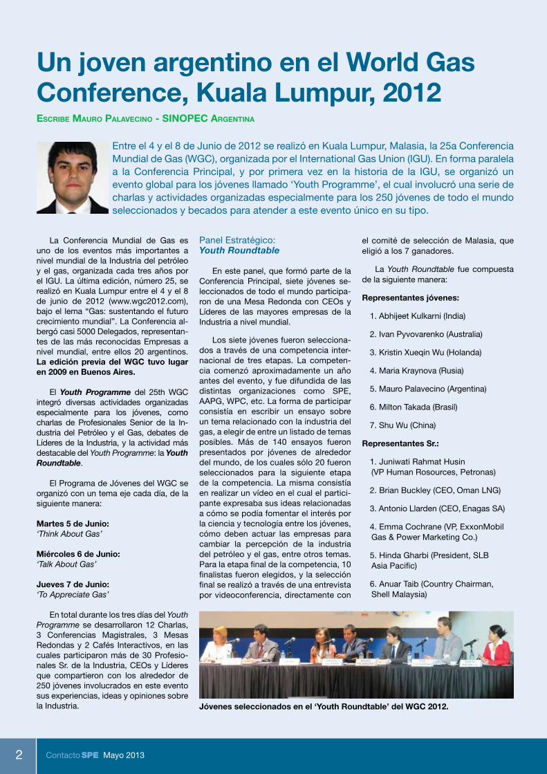
Jóvenes seleccionados en el ‘Youth Roundtable’ del WGC 2012.

Entre el 4 y el 8 de Junio de 2012 se realizó en Kuala Lumpur, Malasia, la 25a Conferencia Mundial de Gas (WGC), organizada por el International Gas Union (IGU). En forma paralela a la Conferencia Principal, y por primera vez en la historia de la IGU, se organizó un evento global para los jóvenes llamado ‘Youth Programme’, el cual involucró una serie de charlas y actividades organizadas especialmente para los 250 jóvenes de todo el mundo seleccionados y becados para atender a este evento único en su tipo.

EscribE mauro Palavecino - sinoPec argentina

Contacto SPE Mayo 2013 3

El Youth Roundtable fue sin dudas el evento más destacado del Programa de Jóvenes del WGC, ya que les dio la posi-bilidad a los jóvenes de exponer sus ideas y sus cuestionamientos sobre diversos temas de la industria ante destacados re-presentantes de las principales empresas a nivel mundial. La Mesa Redonda tuvo lugar en el Plenary Hall del Kuala Lumpur Conventions Center (KLCC), y tuvo una asistencia de unas 500 personas, entre ellos jóvenes participantes del Youth Pro-gramme, Profesionales de la Industria y Delegados de la Conferencia.

Principales charlas y conferencias del Youth Programme

Keynote Address: “The Energy Future is Gas” (Marc Hall, Bayerngas, Alemania)

Durante su presentación hizo princi-palmente hincapié en la importancia que tendrá el gas como recurso en el futuro, al punto de que “no habrá futuro sin gas”. Según Marc Hall la era de los combusti-bles sólidos (carbón) está pronta a termi-nar, la de combustibles líquidos (petróleo) ya ha alcanzado el pico de producción y ha comenzado a declinar, y está comen-zando la era del gas. De ahí la importancia que le otorga a este recurso. Al finalizar su presentación mostró cómo Alemania ase-gura un suministro de gas en todo el año. El suministro de gas que importa Alemania por gasoducto es constante, por lo tanto en épocas de menor consumo (verano), importan más gas del necesario y lo al-macenan en reservorios depletados, para producirlo en épocas de mayor consumo (invierno), y así evitar el desabastecimien-to, o la necesidad de tener que importar gas más caro como podría ser el LNG en forma estacional.

Panel Session: “Evolving Petroleum Professionals in the Gas Industry”

Participantes:

1. Rasik Bahadur, VP Human Resources for Asia, SLB

2. Heike Boss, VP Human Resources, Shell

3. Dr. Jitka Adamkova, Head of Human Resources, RWE Transgas

Moderador: Geert Grieving, Gasterra

En este panel, los líderes de Recursos Humanos de las citadas empresas, ex-pusieron su visión sobre qué buscan las

empresas en los candidatos, cómo es el perfil de las personas que trabajan en la Industria, y cómo hacen las empresas para atraer a más jóvenes, en un contexto de creciente demanda de profesionales de la Industria. Luego se dio lugar a la audien-cia para realizar preguntas a estos líderes, donde los jóvenes pudieron obtener infor-mación, por ejemplo de cómo aplicar para un puesto, cómo ubicarse en la industria o qué distintos caminos existen al momento de empezar una carrera en la Industria del Petróleo y el Gas.

Luncheon Address: “Developing Future Global Gas Leaders” (Klaus Reinisch, CEO Petronas Energy Trading, UK)

Realizó una presentación muy entu-siasta en la cual compartió sus experien-cias de vida y su camino hacia el éxito y desarrollo profesional y personal. Men-cionó 6 “pilares” indispensables para los jóvenes de hoy que quieran convertirse en los líderes del mañana. Los mismos, según Klaus Reinisch, son:

1. Knowledge 2. Sales know-how 3. People Network 4. Think Outside the box 5. Ethics Above All 6. Go International

Klaus Reinisch mencionó como claves del éxito al conocimiento, a siempre saber de lo que se está hablando, a estar siem-pre en contacto con gente y establecer una red de contactos con diversos cole-gas de la Industria, de “pensar fuera de la caja”, o tener pensamiento lateral, a nun-ca olvidarse de la ética tanto profesional como personal, y a salir al mundo. Según Klaus Reinisch, la combinación de estos factores será clave para quienes quieran ser los líderes del mañana, cuando se deberá hablar como mínimo tres idiomas distintos, tener experiencia internacional será casi excluyente, y el mundo sea cada vez más dinámico y competitivo.

Conclusiones

El Youth Programme de la 25a Confe-rencia Mundial de Gas de Kuala Lumpur fue sin lugar a dudas una gran oportuni-dad para todos los jóvenes involucrados de informarse sobre las últimas tecnolo-gías, las tendencias a nivel mundial de la Industria para los próximos años, al mismo tiempo de tener la posibilidad de conocer y establecer contacto con Profe-sionales y jóvenes de la Industria del pe-tróleo y el gas de todo el mundo.

Es interesante destacar la importan-cia que se le otorga en la actualidad a la generación joven en la Industria a nivel mundial, plasmada en esta ocasión por este tan importante evento organizado en forma exclusiva para los jóvenes, que como se mencionó era la primera vez que se realizaba en el marco de un World Gas Conference, pero que sin dudas dejará un precedente para las futuras Conferen-cias. Al mismo tiempo existen diversos eventos similares dedicados especial-mente para los jóvenes, como el Youth Programme del World Petroleum Con-gress, un programa similar que se realiza desde 2008 en el marco del Congreso Mundial de Petróleo organizado cada tres años por el WPC.

Tener la posibilidad de asistir a estos eventos a una temprana edad y en el co-mienzo del desarrollo profesional brinda una oportunidad única de conocer otras culturas, entender el funcionamiento de la Industria a nivel global, y permite una aper-tura no sólo a nivel profesional sino tam-bién personal, que prepara a los jóvenes para entender los desafíos que la Industria encuentra constantemente en un mundo cada día más dinámico y globalizado.

Klaus Reinisch en su presentación ‘Developing Future Global Gas Leaders’

curriculum vitae del ing. mauro Palavecino

Ingeniero Químico graduado de la Univer-sidad Nacional de La Plata, y actualmente estudiante del Posgrado Especialista en Producción de Petróleo y Gas del ITBA. Comenzó su carrera en la Industria hace 2 años, como pasante en SINOPEC Ar-gentina Exploration and Production, Inc., donde actualmente se desempeña como Ingeniero de Reservorios. Paralelamente con sus actividades laborales y acadé-micas, Mauro es miembro de la Comisión de Jóvenes Profesionales del IAPG, de la SPE Argentina, y del comité de jóvenes del World Petroleum Council.


Los Hidratos de Metano: Un recurso cada vez más cercano escribe Patricio a. marshall

Conocidos como curiosidad de laboratorio desde las primeras décadas del siglo XIX, identificados como problemáticos para la producción de hidrocarburos en regiones frías inicialmente y luego en yacimientos offshore, los Hidratos de Metano están en vías de convertirse rápidamente en un recurso energético alter-nativo de gran importancia por la magnitud de su volumen y los avances tecnológicos.

Los Hidratos de Metano, un caso particular de los hidratos de gases, son compuestos naturales conocidos desde el siglo XIX, aunque el interés sobre ellos se ha incrementado en los últimos años.

Son sólidos cristalinos compuestos por agua y un gas (el mas común es Me-tano), estables en condiciones de bajas temperaturas y altas presiones, situación que se da en la naturaleza tanto en los fondos marinos como en algunos po-cos casos en tierra firme, en zonas de altas latitudes, con suelos congelados o “permafrost”. Inicialmente, se los consi-deraba como una curiosidad científica o un inconveniente ingenieril. En efecto, el interés en los hidratos de metano para la industria del petróleo estuvo relacionado con los problemas que ocasionan al de-positarse en las cañerías de producción y transporte disminuyendo el caudal y llegando a obstruir el paso en los con-ductos, generando altas presiones po-tencialmente peligrosas. Debido a esto, ha habido avances en la investigación

de su estructura, propiedades físicas y de técnicas para su remoción. Al mis-mo tiempo, se los comenzó a considerar como potenciales recursos energéticos y también a interpretarlos como un factor importante a tener en cuenta en los es-tudios de Cambio Climático Global y ma-nejo de los gases que provocan el “efecto invernadero”. Un última derivación de las investigaciones se vincula con su capaci-dad potencial como un medio apto para almacenar y transportar gas en barcos.

Presentan la particularidad de pre-sentarse como sólidos cristalinos, si-milares a hielo, y con una composición variable según las condiciones físicas al momento de su formación. Resultan de la combinación de moléculas de agua que se disponen en una estructura reticular de simetría cúbica que alberga en ese re-ticulado moléculas de un gas, este es co-múnmente Metano, pero también puede ser otro hidrocarburo liviano (etano, pro-pano y hasta isobutano), CO

2 y en menor medida otros gases. Genéricamente se

los denomina clatratos, término que en latín significa “enrejado, enjaulado”.

En la naturaleza, los más comunes son combinaciones de metano y agua, por lo que generalmente se toman como sinónimos los términos hidratos de me-tano e hidratos de gases. Como con-secuencia de su composición variable, también lo son sus propiedades físicas, lo que dificulta su estudio y correcta caracterización.

Estudios sobre la composición isotópica de los gases (δ13C) permiten afirmar que su origen puede ser tanto biogénico como termogénico. En este último caso son la expresión de un escape de gas originado en profundidad y entrampado al encon-trar las condiciones de estabilidad de los clatratos. Esta última situación lleva tam-bién a considerar su participación como elemento sello que impide la migración y difusión gaseosa, permitiendo la acumu-lación de gas en trampas estratigráficas no convencionales.

Estructura de los Hidratos de Metano. La unidad estructural mínima, al repetirse en el espacio genera diferentes estructuras cristalinas según sea la composición de los gases participantes en el compuesto ( por ejemplo, sI: Metano, etano, dióxido de carbono, sII Metano con propano, iso-butano, y sH con Metano+neohexano, Metano+ciclopentano..)Molécula de Gas (Metano)

“Jaula” de Moléculas de Agua

S I

S II

S H


Los hidratos se pueden presentar en forma masiva, “cementando” los sedi-mentos, o en forma de láminas o nódulos. Esto depende de las propiedades petro-físicas iniciales de los sedimentos hués-ped (porosidad y permeabilidad) y de las condiciones físico-químicas al momento de su formación (variaciones locales de las condiciones de presión y temperatu-ra, variaciones de salinidad, variaciones en la concentración relativa de los com-ponentes, etc.)

La distribución de sus acumulaciones reconocidas está condicionada exclu-sivamente por la combinación de bajas temperaturas y relativamente altas pre-siones. Hay depósitos de hidratos en tierra firme en regiones de altas latitudes con suelos congelados (Siberia, Alaska y Canadá) pero la mayor proporción de hidratos en la naturaleza se encuentran en fondos marinos a diferentes profun-didades que pueden variar desde cien-tos de metros a más de 1000-2000 m, dependiendo de la proporción de gases (metano y mezclas con etano y otros hi-drocarburos ) que hacen que varíen las condiciones de presión y temperatura ne-cesarias para su estabilidad y existencia.

La identificación de los Hidratos de Metano en el offshore es posible en líneas sísmicas debido a que los sedimentos cementados por los hidratos represen-tan un depósito con muy alta velocidad (aproximadamente 3.3 km/seg, alrededor del doble de la del agua salada) Debajo de las zonas con hidratos las velocidades son menores debido a que los sedimen-tos infrayacentes contienen en sus poros

sólo agua (con velocidad de alrededor de 1.5 km/seg) y a veces incluso gas libre entrampado por la baja permeabilidad de las capas con hidratos. El contraste de velocidad creado entre ambas zonas pro-duce una reflexión muy fuerte cuya traza es paralela a la del fondo marino, y que por ello fue denominada “Reflexión si-muladora del fondo” o en inglés “Bottom Simulating Reflection” (BSR). Ver Figuras a continuación.

Otra característica significativa de los sedimentos que albergan hidratos es el “blanking” o reducción de la amplitud (fuerza) de las reflexiones aparentemente causada por la cementación por los hi-dratos homogeneizando las capas que forman reflectores. Este efecto se produ-ce a lo largo de toda la zona que aloja hi-dratos y puede ser cuantificada para es-timar la cantidad de hidratos presentes.

El factor de expansión al disociarse estos hidratos es un elemento particu-

larmente importante. Un metro cubico de Hidrato de Metano libera al perder el estado sólido alrededor de 164 m3 de metano y 0,8 m3 de agua, e incluso estos valores pueden aumentar, depen-diendo de la eventual presencia de otros hidrocarburos (etano, propano o incluso isobutano, que afectan la estructura re-ticular del hidrato lo que se refleja en la proporción del metano alojado.

Teniendo en cuenta esta caracterís-tica, y como derivación de las investiga-ciones actuales, se está desarrollando tecnología para aprovechar esa capaci-dad de los hidratos de albergar metano en volúmenes importantes como una al-ternativa para el transporte y almacena-miento de gas de una manera económica frente al LNG.

La existencia de hidratos de meta-no está condicionada por los rangos de presión y temperatura a las que son esta-bles. En un gráfico de Presión (o lo que es lo mismo, Profundidad de la columna de agua y sección superior de sedimentos) vs. Temperatura, la línea que une los pun-tos de equilibrio entre el hidrato (sólido) y el gas disuelto, marca esos límites y se puede observar como varían éstos con la profundidad considerada y el gradiente térmico presente.

En el agua, el gradiente térmico varía gradualmente desde la superficie hasta que se estabiliza la temperatura en un va-lor casi constante hasta el fondo marino. A partir de ese punto, comienza a inter-venir el gradiente geotérmico presente en el área.

Se observa que la zona de estabilidad para cada caso (Zona de Estabilidad del Hidrato de Gas o ZEHG), o intervalo de profundidad en que es posible encontrar hidratos, queda definida por dos puntos en la curva de equilibrio: la profundidad del fondo (la presión y la temperatura im-

Areniscas accesibles con la infraestructura existente

Zonas Árticas

Zonas No-ÁrticasFondos Marinos

10x

100x

1000x

???

???

100 000x

Areniscas alejadas de la infraestructura existente

Areniscas de aguas profundas

Reservorios con permeabilidades no significativas

Hidratos superficiales masivos y nodulares someros

Reservorios Marinos con permeabilidad limitada

HM masivos o concentraciones de MH como

nódulos en fangos finos

HM rellenando masivamente pequeñas

fracturas o venillas

HM en granos rellenando el espacio poral del sedimento

Tipo relleno de porosTipo fracturadoTipo masivo o nodular

Nódulos de HM

Rellenos de venillas

por HM

Granos finos de

HM


perantes en la superficie del lecho marino) y la intersección con la curva de gradiente geotérmico. Es evidente que en el caso de gradientes más elevados (pendiente de los segmentos F-G o B-C más suaves) el es-pesor de la ZEHG será menor que en el caso de gradientes más bajos (pendiente más empinada).

Se concluye que la existencia y espe-sor de las zonas donde los hidratos son estables resulta entonces de la combina-ción de: la temperatura del fondo, mag-nitud del gradiente geotérmico, presión hidrostática, composición del gas invo-lucrado y capacidad de los sedimentos como reservorios.

Otros aspectos considerados con respecto a los hidratos de gas en los úl-timos tiempos, es su participación como factor importante a tener en cuenta en los estudios de Cambio Climático Global. El Metano es considerado como el segundo en importancia de los gases que provo-can el “efecto invernadero”, y su libera-ción a partir de depósitos de hidratos de los fondos marinos puede aumentar ese efecto. La situación paradójica produci-

da al aumentar la temperatura media de las masas de agua, o por cambios en la dirección de corrientes cálidas, pueden alterar el gradiente de temperatura y así los depósitos de hidratos estables a una cierta profundidad y temperatura dejarían de serlo, liberando metano, que a su vez provocaría un nuevo aumento de la tem-peratura. Por otro lado, también las varia-ciones en el nivel del mar (y consecuente presión de la columna de agua) afectarían la estabilidad de los hidratos.

También es de remarcar que esas variaciones en las temperaturas de las masas de agua, aun temporarias y loca-lizadas pueden afectar la estabilidad de los hidratos, que al disociarse, hacen que los sedimentos que los contienen pierdan cohesión y puedan producirse desliza-mientos que afectan las instalaciones de fondo de los yacimientos offshore pro-fundos. Un caso excepcional de desliza-miento de fondo marino con remoción de importantes volúmenes de sedimentos fue identificado en Mar del Norte (Storeg-ga) alertando sobre ese potencial peligro para las instalaciones de importantes ya-cimientos cercanos.

Adicionalmente al haberse desarrolla-do una tecnología de producción de me-tano a partir de hidratos, disociándolos y reemplazando el metano por CO2, se ha comenzado a especular sobre el uso de los sitios donde hay hidratos como repo-sitorios secuestrantes de CO2.

Los Hidratos como Recurso Energético

Los Hidratos de Metano actualmente son considerados como los recursos mas abundantes disponibles para la produc-ción de energía. Si bien las estimaciones globales son especulativas y variables según cada informe, representan más del doble de lo asignado a los de Shale Gas (Ver Figura).

Los sistemas de producción conside-rados actualmente se basan en la disocia-ción de los hidratos in situ, mediante algu-no de los siguientes métodos:

1. Calentando el reservorio por en-cima de las temperaturas de estabilidad de los hidratos empleando inyección de agua o vapor.

2. Inyectando inhibidores, tales como metanol o glicol, para disminuir la estabili-dad de esos hidratos, y

3. Disminuyendo la presión del re-servorio por debajo de la de equilibrio, permitiendo la liberación del gas metano contenido.

Los tres métodos son técnicamente posibles, pero los dos primeros presentan resultan a priori antieconómicos. La produc-ción de gas a partir de la despresurización es aun más eficiente al encontrar acumula-ciones de gas libre entrampadas debajo de la capa de hidratos.

Pellets de Hidratos de Metano, que permitirían su transporte en modo seguro y económico desde instalaciones en alta mar.

Fondo Marino

Hidratos de Gas

Base de la Zona de Estabilidad de Hidratos de Gas(GHSZ)

Gas Libre

2.01.50

100

Profundidad(m.b.f.m.)

200

300

400

Vp (km/s)

Base de la zona de Gas Libre(FGZ)

Respuesta Sísmica

BS

R

GHSZ

FGZ

Sitio 1248

Fondo del mar

Tiem

po

de

viaj

e en

dos

dire

ccio

nes

(s)

BSR

Y

A

250 m

1.3 1.3

1.2 1.2

1.1 1.1


Gráfico de estabilidad de hidratos de metano. El espesor de la zona de estabilidad o formación de los Hidratos de Metano en fondos marinos es dependiente de la profundidad de agua (Presión) y el gradiente geotérmico (Temperatura) En el caso del gráfico, para un mismo Gradiente Geotérmicol (F-G = B-C) a diferente profundidad de agua es posible tener diferentes espesores de Zona de Estabilidad de Hidratos.

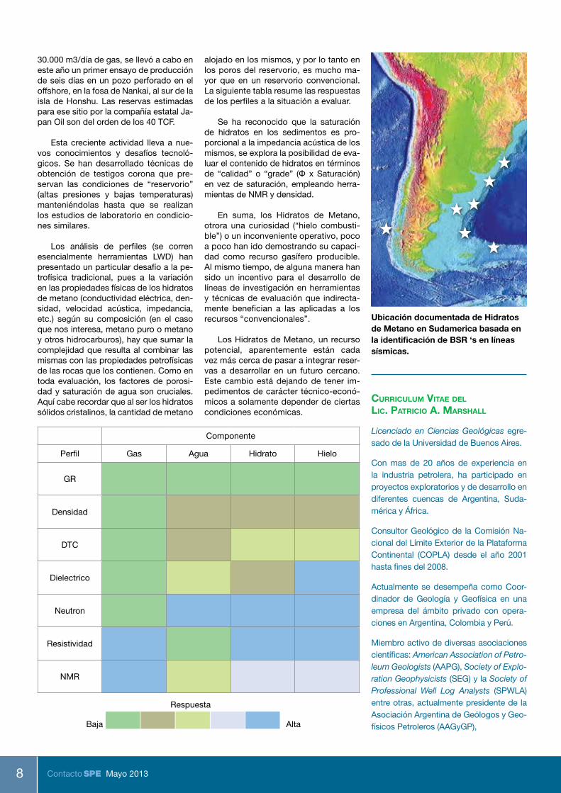
En el caso particular de nuestro país, dadas las características geográficas de Argentina, la existencia de Hidratos de Me-tano solo puede esperarse en el offshore, donde ya se ha documentado su existen-cia en registros sísmicos. Esta situación en mayor o menor medida se aplica tam-bién al resto de los países de Sudamérica, como se observa en la Figura siguiente.

Hay avances que permiten estimar que en algunos casos se podrán poner en pro-ducción en un futuro muy cercano algu-nas de las acumulaciones estudiadas. Las

primeras experiencias se han logrado en proyectos llevados a cabo por consorcios internacionales (combinación de organis-mos de investigación y compañías esta-tales de Estados Unidos, Japón, Canadá, Alemania, India y otros países, universida-des, y compañías de servicios de la indus-tria petrolera) desarrollados en tierra firme, en Alaska (Proyecto Mallik).

En el año 2002 se llevó a cabo el primer ensayo por disociación a partir de calenta-miento por agua, y se lograron recuperar 470 m3 de gas en 123,7 horas.

En año 2007 se ensayó por despresuri-zación, recuperando 830 m3 de gas en 12,5 horas, y se repitió el ensayo por el mismo método durante 6 días, recuperando un to-tal de 13.000 m3 de gas, con flujos de 2000 a 4000 m3/día.

Los avances hacen que proyectos que antes eran subeconómicos ya son consi-derados marginales o cercanos a ser eco-nómicamente viables.

En Japón, luego de simulaciones que consideraban factibles flujos de 9000 a

Shale Gas19%

Hidratos de Metano

19%

Tar Sands 0%Heavy Oils 0%

Oil Shale19%

CBM11%

Tight9%

MethanolSteam oHot Water

Inhibitor InjectionThermal InjectionDepressurization

Gas Out

Gas Out

Gas Out

Hydrate Imperm. Imperm.

Hydrate Hydrate

Impermeable Rock Impermeable Rock

Dissociated

Free-Gas

Hydrate

Reservoir

Cap Rock Rock

Dissociated HydrateDissociated Hydrate

Pro

fund

idad

de

agua

(m) =

Pre

sión

Gradiente Térmico en el Agua

D0

400

800

1200

1600

2000-10 0 10 20

A

G

C

F

Hidrato de CH4 Equilibrium

Hidratos

Gas

Fondo Caso 2

300

m

200

mFondo Caso 1

Zon

a d

e E

stab

ilid

ad d

e H

idra

tos

de

CH

4

Gradiente Geotérmico

B

Recursos de Hidrocarburos


30.000 m3/día de gas, se llevó a cabo en este año un primer ensayo de producción de seis días en un pozo perforado en el offshore, en la fosa de Nankai, al sur de la isla de Honshu. Las reservas estimadas para ese sitio por la compañía estatal Ja-pan Oil son del orden de los 40 TCF.

Esta creciente actividad lleva a nue-vos conocimientos y desafíos tecnoló-gicos. Se han desarrollado técnicas de obtención de testigos corona que pre-servan las condiciones de “reservorio” (altas presiones y bajas temperaturas) manteniéndolas hasta que se realizan los estudios de laboratorio en condicio-nes similares.

Los análisis de perfiles (se corren esencialmente herramientas LWD) han presentado un particular desafío a la pe-trofísica tradicional, pues a la variación en las propiedades físicas de los hidratos de metano (conductividad eléctrica, den-sidad, velocidad acústica, impedancia, etc.) según su composición (en el caso que nos interesa, metano puro o metano y otros hidrocarburos), hay que sumar la complejidad que resulta al combinar las mismas con las propiedades petrofísicas de las rocas que los contienen. Como en toda evaluación, los factores de porosi-dad y saturación de agua son cruciales. Aquí cabe recordar que al ser los hidratos sólidos cristalinos, la cantidad de metano

alojado en los mismos, y por lo tanto en los poros del reservorio, es mucho ma-yor que en un reservorio convencional. La siguiente tabla resume las respuestas de los perfiles a la situación a evaluar.

Se ha reconocido que la saturación de hidratos en los sedimentos es pro-porcional a la impedancia acústica de los mismos, se explora la posibilidad de eva-luar el contenido de hidratos en términos de “calidad” o “grade” (Φ x Saturación) en vez de saturación, empleando herra-mientas de NMR y densidad.

En suma, los Hidratos de Metano, otrora una curiosidad (“hielo combusti-ble”) o un inconveniente operativo, poco a poco han ido demostrando su capaci-dad como recurso gasífero producible. Al mismo tiempo, de alguna manera han sido un incentivo para el desarrollo de líneas de investigación en herramientas y técnicas de evaluación que indirecta-mente benefician a las aplicadas a los recursos “convencionales”.

Los Hidratos de Metano, un recurso potencial, aparentemente están cada vez más cerca de pasar a integrar reser-vas a desarrollar en un futuro cercano. Este cambio está dejando de tener im-pedimentos de carácter técnico-econó-micos a solamente depender de ciertas condiciones económicas.

Ubicación documentada de Hidratos de Metano en Sudamerica basada en la identificación de BSR ‘s en líneas sísmicas.

Componente

Perfil Gas Agua Hidrato Hielo

GR

Densidad

DTC

Dielectrico

Neutron

Resistividad

NMR

Respuesta

Baja Alta

curriculum vitae del lic. Patricio a. marshall

Licenciado en Ciencias Geológicas egre-sado de la Universidad de Buenos Aires.

Con mas de 20 años de experiencia en la industria petrolera, ha participado en proyectos exploratorios y de desarrollo en diferentes cuencas de Argentina, Suda-mérica y África.

Consultor Geológico de la Comisión Na-cional del Límite Exterior de la Plataforma Continental (COPLA) desde el año 2001 hasta fines del 2008.

Actualmente se desempeña como Coor-dinador de Geología y Geofísica en una empresa del ámbito privado con opera-ciones en Argentina, Colombia y Perú.

Miembro activo de diversas asociaciones científicas: American Association of Petro-leum Geologists (AAPG), Society of Explo-ration Geophysicists (SEG) y la Society of Professional Well Log Analysts (SPWLA) entre otras, actualmente presidente de la Asociación Argentina de Geólogos y Geo-físicos Petroleros (AAGyGP),


©2013 Schlumberger. 13-UG-0003

slb.com/shale

¿Cuán consistente puede esperarse que sea la producción de estos pozos de shale?

En los pozos con recursos no convencionales, los registros de producción indican que un 40% de los grupos de disparos no contribuye a la producción. La experiencia adquirida en más de 20 000 pozos de todas las extensiones productivas de shale activas en el mundo nos ha enseñado que la identificación y la estimulación de las zonas correctas requiere mediciones precisas, un entorno de colaboración, aplicaciones de computación analíticas y tecnologías de estimulación innovadoras. Permítanos ayudarlo a convertir mayor comprensión en mejor producción.

Las rocas heterogéneas nunca producirán resultados homogéneos.


Luis Alberto Rey nació en Buenos Aires el 24 de Diciembre de 1929 y falleció en el año 2005, a los 75 años de edad. Fue el fundador y presidente de Pluspetrol, la tercer empresa operadora en el upstream nacional si se la mide por su producción, y es además, una de las pocas compañías del sector de capital totalmente argentino. Presidió el Club del Petróleo desde el año 1994 hasta su fallecimiento. Se casó en 1960 con Edith Rodríguez, que lo compa-ñó durante toda su vida y con quien tuvo tres hijos.

Nacido en el seno de una familia de cla-se media, cursa el secundario en el colegio nacional Mariano Moreno y se recibe de in-geniero civil en la Facultad de Ingeniería de la Universidad de Buenos Aires en 1956. En 1955 Rey había sido elegido Presidente del Centro de Estudiantes de Ingeniería (CEI) La Linea Recta, único órgano que repre-sentaba entonces a los estudiantes y que operaba en clandestinidad como parte de la FUBA. El apoyo del CEI a la Intervención de la Facultad dispuesta por el Gobierno que asumió en ese año resultó básico para

con el gas natural durante toda su carrera empresarial: a Clark Bros le siguen Tauro y luego, en el upstream del gas, Centenario, Ramos, Bolivia y finalmente en su mayor logro empresarial: Camisea, en el Perú.

En 1976, se inicia en el upstream pe-trolero fundando Pluspetrol S.A., vía la cual gana, por licitación, áreas que YPF ofrecía a compañías argentinas para mejorar su explotación, siendo la primera Centenario, situada en Neuquén. Al año siguiente y por la misma vía Pluspetrol obtiene el área Ra-mos, en Salta. Esta área, principalmente gasífera, lleva a Pluspetrol a involucrarse mas profundamente en el gas, a explorar en Bolivia y resulta fundamental para ac-ceder más tarde al área Camisea, donde Pluspetrol probó su capacidad operativa en condiciones de aislación y extrema du-reza geográfica.

En el año 1979 Pluspetrol emprende su expansión internacional con negocios en Colombia y Costa de Marfil, más tarde en el año 1990, abre oficinas de represen-tación en Houston, Estados Unidos, y co-menzó a explorar en Bolivia.

En 1994 inicia actividades en Argelia y Túnez y en 1996 llega a Perú, donde em-prendió el desarrollo del área de Camisea, con el mayor yacimiento de gas de América del Sur, y el subsiguiente desarrollo del mer-cado de gas de Perú, involucrándose en el transporte y la distribución del gas en Lima, modificando en forma sustancial la matriz energética de ese país. Esta tarea exitosa-mente cumplida y de carácter pionero, le otorgó a Pluspetrol la categoría y respeto de operador petrolero a nivel internacional. En Camisea Shell había descubierto gas en el 1986, que luego abandonó al no encontrar la solución económica para su desarrollo. Fue Rey quien lideró un consorcio en el cual Pluspetrol fue (y es) el operador, y cuyo pro-yecto fue aceptado por el gobierno peruano. Perú confío en Rey y viceversa: fue un clá-sico caso de “win win”. Hoy Camisea pro-

reencauzar el orden y la calidad de la en-señanza en esa Facultad, ordenando los planes de exámenes y eliminando la poli-tización en su cuerpo lectivo.

A pocos meses de haberse recibido se fue a New York, EEUU, donde encuen-tra trabajo como ingeniero de proyecto y desarrollo de turbinas y compresores de gas en Clark Bros Co, compañía del grupo Dresser, radicada en la ciudad de Olean, en el estado de Nueva York.

Tres años después, en 1959 regresa a Argentina como gerente regional de Dresser Industries, compañía especiali-zada en equipamiento para la industria petrolera. A poco de llegar a la Argentina, en 1964, funda Tauro S.A., empresa de construcciones civiles e industriales de la cual fue presidente. Tauro instala varias plantas de compresión de gas en los ga-soductos en construcción, acercándose así al quehacer gasífero.

Aquel primer empleo resultó premoni-torio: Rey estaría vinculado íntimamente

Luis Rey y Pluspetrol Una historia argentina

PRODUCCIÓN DE PETROLEO OPERADO 65% PROPIO

PRODUCCIÓN DE GAS OPERADO 65% PROPIO

6,500

7,000,000

PRODUCCIÓN NACIONALORDEN PRODUCTOR NACIONAL

3RO 7%

5.5%5TO

Pluspetrol en la Argentina

PRODUCCIÓN (m3/día)


vee de gas a Lima y exporta componentes pesados del gas (NGL) generando divisas para Perú. Para ello se construyeron dos gasoductos con un total de 1250 Kms de longitud cruzando los Andes: uno a la ciu-dad portuaria de Pisco, donde se carga el NGL para su exportación, el otro para abastecer a Lima. (Google cubre la historia de este proyecto)

En 1996, Pluspetrol se inició en el ne-gocio de la generación eléctrica en Tucu-mán y al año siguiente ingresó en la distri-bución de gas en Brasil.

En el año 2004 fue condecorado con la orden “Al mérito por servicios distinguidos” en el grado de Gran Oficial por el gobierno de Perú en una emotiva ceremonia realizada en su domicilio en el Club Pingüinos, dado que su delicado estado de salud le impedía viajar a Lima. Fue en reconocimiento a ha-ber liderado el cambio de su la matriz ener-gética al que introdujo, vía Camisea, a su condición de moderno país gasífero. Para esta Ceremonia viajaron de Lima los minis-tros de Energía y de Relaciones exteriores de Perú, en representación de su Presidente Alejandro Toledo Manrique.

Rey ejercía un liderazgo nato que se manifestó en todos sus emprendimien-tos, donde su aporte era de gestarlos para luego de encabezarlos. Así fue que Pluspetrol ha sido y es operador en to-dos sus emprendimientos energéticos, a veces incluso siendo un accionista mi-noritario. Pluspetrol opera o ha operado en consorcios donde participaban com-pañías de mayor porte que ella, como Exxon, Mobil, Hunt Oil, Primary Fuels, Techint/Tecpetrol y otros.

Destacaba Rey la importancia de la perseverancia, virtud que practicaba cons-tantemente. Era una persona de objetivos muy claros que entusiasmaba a quien tra-bajaba con él porque desde el comienzo lo hacía sentir que formaba parte del proyec-

pecialmente delicado y manejado con un mínimo de inconvenientes por Pluspetrol. El área, cercana a la Reserva Nahua-Nanti, tenía una historia de malas experiencias desde la época de la explotación del cau-cho y además existían en sus cercanías tribus sin contacto aún con la modernidad. Se llegó a acuerdos exitosos y se firmaron convenios destinados a respetar el ecosis-tema social y ecológico y bajo esta protec-ción se desarrollaron las operaciones sin problemas ambientales.

Pluspetrol es el resultado de la ges-tión de un empresario producto neto de su terruño, que con visión y coraje mostró que aún en condiciones difíciles es posible crear y crecer. Un ejemplo que merece ins-pirar a sus compatriotas.

Entrevistas al Dr. Alberto Selasco vi-cepresidente de Pluspetrol hasta su retiro en el año 1997, al Ingeniero Juan Carlos Pisanu: Ingreso a Pluspetrol en 1981, y en la actualidad es miembro de su directorio y al Ing. Oscar Secco; Director y Gerente General: 1981 -1993, Investigación y reco-pilación Dra. Magali Sol Giovanelli Petito.

to. Se caracterizó por estar presente en los momentos críticos de la empresa. En un “blow out” de un pozo exploratorio en Bo-livia y que fue uno de los accidentes más riesgosos que tuvo la empresa, en ese mo-mento de incertidumbre Rey voló sorpresi-va y rápidamente a la locación para alentar y dar su apoyo a quienes tenían la difícil tarea de contener la surgencia.

La crisis financiera del año 2001 com-plicó el proyecto. El panorama era doble-mente desafiante, ya que además de las finanzas existía la complejidad desde el punto de vista técnico, pero de todos mo-dos se llevo a cabo exitosamente.

Asimismo aportaron al éxito del pro-yecto las alianzas estratégicas que pudie-ran apalancar el crecimiento de la empre-sa, socios que no solo aportaran capital, sino que trajeran experiencia, dado que se operó en la selva, en un ámbito diferente al habitual, especialmente con una logística que exigió el uso de los grandes ríos ama-zónicos y de helicópteros para transportar los equipos pesados al área. El manejo de la parte ambiental, tanto en su aspecto na-tural como en el de sus habitantes, fue es-

Luis Rey. Condecoración con la Orden “AL MERITO POR SERVICIOS DISTINGUIDOS” EN EL GRADO DE GRAN OFICIAL , otorgada por el Gobierno del Perú. 12 Septiembre 2004.

Mipaya

Pagoreni

San Martín

Cashiriari

Pluspetrol • Hunt Oil • SK Corp. • YPF • Tecpetrol • Sonatrach

Socios en el Yacimiento

23 PRODUCTORES

PozosYACIMIENTOS

CUSCO PERÚ

INYECTORES5

GAS LÍQUIDOS

Producción ( m3/día):

50,000,000 17,000

Consumo Local

NGL

Reinyección30

40

30

Destino producción de gas (%)

Área Camisea, Depto. Cuzco, Perú


Un grupo que integraban Oscar Alvarez, Gustavo Califa-no, Daniel Herbalejo, Claudio Moreno, Jorge Persini, Robert Steven y Hugo Carranza, toman en 2002 la decisión de cons-truir un espacio en el ámbito nacional para el desarrollo de modelos de simulación y de convocar a una primera reunión en el transcurso de ese año. Casi como una necesidad se formó para facilitar el intercambio de información sobre el desarrollo de modelos de simulación y optimización de redes en sistemas de transporte y distribución de hidrocarburos. Promover el conocimiento de tecnologías aplicadas y expe-riencias de la región.

El Grupo de Interés en Modelado y Operación de Redes y Ductos GIMOR, auspiciado por la SPE de Argentina y algunas empresas del rubro, se oriento a especialistas vinculados a la actividad por su participación en empresas de transporte, dis-tribución de petróleo y gas, universidades y consultores que acrediten experiencia en la materia. Cada año culminaba con una jornada de presentación de ponencias con la asistencia de más de 100 interesados. El GIMOR continuó hasta el año 2009 habiendo realizado 8 reuniones anuales y más de 50 tra-bajos presentados.

Síntesis de la Conferencia del 22 de Octubre Gas Pipeline Simulation, fundamentals and state of art Introduction Flow in high pressure gas networks is unsteady. Conditions are always changing with time, no matter how small some of the changes may be. Dynamic models are just a particular class of a differential equation model in which time derivatives are present. During transport of gas in pipelines the gas stream loses a part of its initial energy due to frictional resistance which results in a loss of pressure. This is compensated for by compressors installed in compressor stations.

Compression of the gas has the undesired side effect of heating the gas.

The gas may have to be cooled: to prevent damage to the main transmission pipeline, to improve the efficiency of the ove-rall compression process. (Always it is a matter of balancing ca-pital and maintenance costs against operating costs).

The transient flow of gas in pipes can be adequately des-cribed by a one dimensional approach. The basic equations describing the transient flow of gas in pipes are derived from an equation of motion (or momentum), an equation of continui-ty, equation of energy and state equation.

In practice the form of the mathematical models varies with the assumptions made as regards the conditions of operation of the networks. In much of the literature, either an isother-mal or an adiabatic approach is adopted. For the case of slow transients caused by fluctuations in demand, it is assumed that the gas in the pipe has sufficient time to reach thermal equilibrium with its constant - temperature surroundings.

When rapid transients were under consideration, it was as-sumed that the pressure changes occurred instantaneously, allowing no time for heat transfer to take place between the gas in the pipe and the surroundings. Adiabatic flow relates to fast dynamic changes in the gas. For many dynamic gas applications this assumption that a process has a constant temperature or is adiabatic is not valid. In this case, tempera-ture of gas is a function of distance and is calculated using a mathematical model which includes energy equation.

Mathematical models for transient flow of gas in the pipes

Conservation of mass: continuity equation

Generally, the continuity equation is expressed in the form:

where: w - flow velocity, ρ - density of gas

Substituting M = ρ w A, we have:

where: A - cross-section area of the pipe, M - mass flow

Síntesis de la Conferencia del 22 de Octubre

Gas Pipeline Simulation Fundamentals and the State of the Art

Introduction Flow in high pressure gas networks is unsteady. Conditions are always changing with time, no matter how small some of the changes may be. Dynamic models are just a particular class of a differential equation model in which time derivatives are present. During transport of gas in pipelines the gas stream loses a part of its initial energy due to frictional resistance which results in a loss of pressure. This is compensated for by compressors installed in compressor stations. Compression of the gas has the undesired side effect of heating the gas. The gas may have to be cooled: to prevent damage to the main transmission pipeline, to improve the efficiency of the overall compression process. (Always it is a matter of balancing capital and maintenance costs against operating costs). The transient flow of gas in pipes can be adequately described by a one dimensional approach. The basic equations describing the transient flow of gas in pipes are derived from an equation of motion (or momentum), an equation of continuity, equation of energy and state equation. In practice the form of the mathematical models varies with the assumptions made as regards the conditions of operation of the networks.In much of the literature, either an isothermal or an adiabatic approach is adopted. For the case of slow transients caused by fluctuations in demand, it is assumed that the gas in the pipe has sufficient time to reach thermal equilibrium with its constant - temperature surroundings. When rapid transients were under consideration, it was assumed that the pressure changes occurred instantaneously, allowing no time for heat transfer to take place between the gas in the pipe and the surroundings. Adiabatic flow relates to fast dynamic changes in the gas. For many dynamic gas applications this assumption that a process has a constant temperature or is adiabatic is not valid. In this case, temperature of gas is a function of distance and is calculated using a mathematical model which includes energy equation. Mathematical models for transient flow of gas in the pipes Conservation of mass: continuity equation Generally, the continuity equation is expressed in the form: where: w - flow velocity, ρ - density of gas Substituting M = ρ w A, we have: where: A - cross-section area of the pipe, M - mass flow Newton's second law of motion: momentum equation The basic form of momentum equation can be expressed in the form: where: f - Fanning friction coefficient, g-the net body force per unit mass (the acceleration of gravity) and a - the angle between the horizon and the direction x.

The constituent factors define the gas inertia, hydraulic friction force, force of gravity and the flowing gas dynamic pressure respectively. State equation An equation of state for a gas relates the variables p, ρ, and T. The type of equation which is commonly used in the gas industry is: where the deviation from the ideal gas law is absorbed in the compression factor Z. Conservation of the energy The basic form of energy equation is the following:

( )ρ ρ∂ ∂− =

∂ ∂

wx t

ρ∂ ∂− =

∂ ∂

MA x t1

( ) ( )ρρρρ α

∂∂∂− − − = +∂ ∂ ∂

sinwwp f w g

x D t x

222

( )( )( )/ ,t wρ∂ ∂ ( )22 / ,f w Dρ ( )sin ,gρ α ( )( )( )2/ x wρ∂ ∂

ρ=

p ZRT

( )ρ ρ ρρ

⎡ ⎤ ⎡ ⎤⎛ ⎞ ⎛ ⎞∂ ∂= + + + + + +⎢ ⎥ ⎢ ⎥⎜ ⎟ ⎜ ⎟∂ ∂⎝ ⎠ ⎝ ⎠⎣ ⎦ ⎣ ⎦

v vw p wq c T gz w c T gz

t x

2 2

2 2





( )ρ ρ∂ ∂− =

∂ ∂

wx t

ρ∂ ∂− =

∂ ∂

MA x t1

( ) ( )ρρρρ α

∂∂∂− − − = +∂ ∂ ∂

sinwwp f w g

x D t x

222


ρ=

p ZRT

( )ρ ρ ρρ

⎡ ⎤ ⎡ ⎤⎛ ⎞ ⎛ ⎞∂ ∂= + + + + + +⎢ ⎥ ⎢ ⎥⎜ ⎟ ⎜ ⎟∂ ∂⎝ ⎠ ⎝ ⎠⎣ ⎦ ⎣ ⎦


t x

2 2

2 2

El Dr. Andrzej Osiadacz ofreció el 22 de octubre de 2012 una conferencia en su paso por Buenos Aires. Los memoriosos aún recuerdan aquel excelente curso que dictó en Buenos Aires del 5 al 9 de Noviembre del 2001. El curso de 2001 fue de tal nivel que la mayor parte de los especialistas que asistimos nos preguntamos cómo era posible darle continuidad al conocimiento especializado en flujo de fluidos compresibles en un país cuya matriz energética está soportada en un 50% en el Gas Natural.

Conferencia de Andrzej Osiadacz

Gas pipeline simulation, fundamentals and state of art


Newton’s second law of motion: momentum equation

The basic form of momentum equation can be expressed in the form:

where: f - Fanning friction coefficient, g-the net body force per unit mass (the acceleration of gravity) and a - the angle between the horizon and the direction x.

The constituent factors

define the gas inertia, hydraulic friction force, force of gravity and the flowing gas dynamic pressure respectively.

State equation

An equation of state for a gas relates the variables p, ρ, and T. The type of equation which is commonly used in the gas industry is:

where the deviation from the ideal gas law is absorbed in the compression factor Z.

Conservation of the energy

The basic form of energy equation is the following:

where: q - the heat addition per unit mass per unit time, T - gas temperature, cV - specific heat at constant volume.

The following assumptions are made in developing the equations for transient gas flow in pipeline:

• for one dimensional flow of gas, pressure, density, velocity and etc, are only functions of time and the distance along the axis of the pipe,

• ρ, p, w, and T of the gas can be adequately described by their average values over the cross - section,

• the cross sectional area is constant along the path of stream of gas,

• expansion at pipe wall may be neglected,

• - the gas compressibility is assumed constant over the range of a single problem,

• the radius of curvature of the pipe is large in comparison to diameter,





( )ρ ρ∂ ∂− =

∂ ∂

wx t

ρ∂ ∂− =

∂ ∂

MA x t1

( ) ( )ρρρρ α

∂∂∂− − − = +∂ ∂ ∂

sinwwp f w g

x D t x

222


ρ=

p ZRT

( )ρ ρ ρρ

⎡ ⎤ ⎡ ⎤⎛ ⎞ ⎛ ⎞∂ ∂= + + + + + +⎢ ⎥ ⎢ ⎥⎜ ⎟ ⎜ ⎟∂ ∂⎝ ⎠ ⎝ ⎠⎣ ⎦ ⎣ ⎦


t x

2 2

2 2





( )ρ ρ∂ ∂− =

∂ ∂

wx t

ρ∂ ∂− =

∂ ∂

MA x t1

( ) ( )ρρρρ α

∂∂∂− − − = +∂ ∂ ∂

sinwwp f w g

x D t x

222


ρ=

p ZRT

( )ρ ρ ρρ

⎡ ⎤ ⎡ ⎤⎛ ⎞ ⎛ ⎞∂ ∂= + + + + + +⎢ ⎥ ⎢ ⎥⎜ ⎟ ⎜ ⎟∂ ∂⎝ ⎠ ⎝ ⎠⎣ ⎦ ⎣ ⎦


t x

2 2

2 2





( )ρ ρ∂ ∂− =

∂ ∂

wx t

ρ∂ ∂− =

∂ ∂

MA x t1

( ) ( )ρρρρ α

∂∂∂− − − = +∂ ∂ ∂

sinwwp f w g

x D t x

222


ρ=

p ZRT

( )ρ ρ ρρ

⎡ ⎤ ⎡ ⎤⎛ ⎞ ⎛ ⎞∂ ∂= + + + + + +⎢ ⎥ ⎢ ⎥⎜ ⎟ ⎜ ⎟∂ ∂⎝ ⎠ ⎝ ⎠⎣ ⎦ ⎣ ⎦


t x

2 2

2 2





( )ρ ρ∂ ∂− =

∂ ∂

wx t

ρ∂ ∂− =

∂ ∂

MA x t1

( ) ( )ρρρρ α

∂∂∂− − − = +∂ ∂ ∂

sinwwp f w g

x D t x

222


ρ=

p ZRT

( )ρ ρ ρρ

⎡ ⎤ ⎡ ⎤⎛ ⎞ ⎛ ⎞∂ ∂= + + + + + +⎢ ⎥ ⎢ ⎥⎜ ⎟ ⎜ ⎟∂ ∂⎝ ⎠ ⎝ ⎠⎣ ⎦ ⎣ ⎦


t x

2 2

2 2

Generally, the transient isothermal flow of gas in a pipe is described by the system of equations), i.e.

This represents a system of two first-order non-linear partial differential equations hyperbolic type for the three state varia-bles, p, r, and w. The necessary third equation is the gas law.

For the transient non-isothermal flow the temperature profile is a function of pipeline distance. In this case the transient, non-isothermal flow of gas in a horizontal pipe

is described by the system of equations: - conservation of mass, - momentum equation, - state equation, - energy equation.

The simplified models for gas obtained by neglecting some terms in the basic equations

Two contradictory constraints are imposed on the basic equa-tions It is required that on the one hand the description of the phenomenon is accurate, and on the other that it is enough simple so that the computational means necessary for sol-ving this model is reasonable. As a rule simplified models are sought which present a reasonable compromise between the accuracy of description and the costs of solution

The simplified models are obtained by neglecting some terms in the basic equations as a result of a quantitative estimation of the particular elements of the equation for some given condi-tions of operation of the pipeline. This means that the model of transient flow used for similation should be fitted to the given conditions of operation of the pipe

Assuming that:

are small when compared to the other terms and may be discarded for horizontally lie pipes momentum equation takes the form:

Above equations are a set of non-linear, parabolic partial differen-tial equations in p, r and w, with independent variables x and t.

Equations can be written in the form

where: q - the heat addition per unit mass per unit time,T - gas temperature, cV - specific heat at constant volume. The following assumptions are made in developing the equations for transient gas flow in pipeline:


• ρ, p, w, and T of the gas can be adequately described by their average values over the cross - section, • the cross sectional area is constant along the path of stream of gas, • expansion at pipe wall may be neglected, • - the gas compressibility is assumed constant over the range of a single problem, • the radius of curvature of the pipe is large in comparison to diameter,

Generally, the transient isothermal flow of gas in a pipe is described by the system of equations), i.e. where and This represents a system of two first-order non-linear partial differential equations hyperbolic type for the three state variables, p, r, and w. The necessary third equation is the gas law. For the transient non-isothermal flow the temperature profile is a function of pipeline distance. In this case the transient, non-isothermal flow of gas in a horizontal pipe is described by the system of equations:

- conservation of mass, - momentum equation, - state equation, - energy equation.

The simplified models for gas obtained by neglecting some terms in the basic equations Two contradictory constraints are imposed on the basic equations It is required that on the one hand the description of the phenomenon is accurate, and on the other that it is enough simple so that the computational means necessary for solving this model is reasonable. As a rule simplified models are sought which present a reasonable compromise between the accuracy of description and the costs of solution The simplified models are obtained by neglecting some terms in the basic equations as a result of a quantitative estimation of the particular elements of the equation for some given conditions of operation of the pipeline. This means that the model of transient flow used for similation should be fitted to the given conditions of operation of the pipe Assuming that: and are small when compared to the other terms and may be discarded for horizontally lie pipes momentum equation takes the form: Above equations are a set of non-linear, parabolic partial differential equations in p, r and w, with independent variables x and t. Equations can be written in the form Taking into account that M = rwA = rQ = rs Qs (where subscript s indicates values under Standard Conditions) and p=c2ρ the above system of equations takes the form

( ) 02 =+xwc

tp

∂ρ∂

∂∂ ρ/pc =

( ) ( ) 0sin2 22

=−−−−− wt

wx

gDwf

xp

ρ∂∂

ρ∂∂

αρρ

∂∂

ρ α =sin ,g 0 ( )( )/ 0x wgzρ∂ ∂ =

( )xw∂ρ∂ 2 ( )

tw

∂ρ∂

02 2

=+Dwf

xp ρ∂∂ ( )

⎪⎪⎭

⎪⎪⎬

⎫

=+

=+

02

0

2

2

Dwf

xp

xwc

tp

ρ∂∂

∂ρ∂

∂∂

⎪⎪⎭

⎪⎪⎬

⎫

=+

=+

02

0

2

2

Dwf

xp

xM

tp

cA

ρ∂∂

∂∂

∂∂

⎪⎪

⎭

⎪⎪

⎬

⎫

−=

⋅−=

pDAQcf

xp

xQ

Ac

tp

s

ss

2

222

2

2 ρ

∂∂

∂∂ρ

∂∂







( ) 02 =+xwc

tp

∂ρ∂

∂∂ ρ/pc =

( ) ( ) 0sin2 22

=−−−−− wt

wx

gDwf

xp

ρ∂∂

ρ∂∂

αρρ

∂∂

ρ α =sin ,g 0 ( )( )/ 0x wgzρ∂ ∂ =

( )xw∂ρ∂ 2 ( )

tw

∂ρ∂

02 2

=+Dwf

xp ρ∂∂ ( )

⎪⎪⎭

⎪⎪⎬

⎫

=+

=+

02

0

2

2

Dwf

xp

xwc

tp

ρ∂∂

∂ρ∂

∂∂

⎪⎪⎭

⎪⎪⎬

⎫

=+

=+

02

0

2

2

Dwf

xp

xM

tp

cA

ρ∂∂

∂∂

∂∂

⎪⎪

⎭

⎪⎪

⎬

⎫

−=

⋅−=

pDAQcf

xp

xQ

Ac

tp

s

ss

2

222

2

2 ρ

∂∂

∂∂ρ

∂∂







( ) 02 =+xwc

tp

∂ρ∂

∂∂ ρ/pc =

( ) ( ) 0sin2 22

=−−−−− wt

wx

gDwf

xp

ρ∂∂

ρ∂∂

αρρ

∂∂

ρ α =sin ,g 0 ( )( )/ 0x wgzρ∂ ∂ =

( )xw∂ρ∂ 2 ( )

tw

∂ρ∂

02 2

=+Dwf

xp ρ∂∂ ( )

⎪⎪⎭

⎪⎪⎬

⎫

=+

=+

02

0

2

2

Dwf

xp

xwc

tp

ρ∂∂

∂ρ∂

∂∂

⎪⎪⎭

⎪⎪⎬

⎫

=+

=+

02

0

2

2

Dwf

xp

xM

tp

cA

ρ∂∂

∂∂

∂∂

⎪⎪

⎭

⎪⎪

⎬

⎫

−=

⋅−=

pDAQcf

xp

xQ

Ac

tp

s

ss

2

222

2

2 ρ

∂∂

∂∂ρ

∂∂







( ) 02 =+xwc

tp

∂ρ∂

∂∂ ρ/pc =

( ) ( ) 0sin2 22

=−−−−− wt

wx

gDwf

xp

ρ∂∂

ρ∂∂

αρρ

∂∂

ρ α =sin ,g 0 ( )( )/ 0x wgzρ∂ ∂ =

( )xw∂ρ∂ 2 ( )

tw

∂ρ∂

02 2

=+Dwf

xp ρ∂∂ ( )

⎪⎪⎭

⎪⎪⎬

⎫

=+

=+

02

0

2

2

Dwf

xp

xwc

tp

ρ∂∂

∂ρ∂

∂∂

⎪⎪⎭

⎪⎪⎬

⎫

=+

=+

02

0

2

2

Dwf

xp

xM

tp

cA

ρ∂∂

∂∂

∂∂

⎪⎪

⎭

⎪⎪

⎬

⎫

−=

⋅−=

pDAQcf

xp

xQ

Ac

tp

s

ss

2

222

2

2 ρ

∂∂

∂∂ρ

∂∂







( ) 02 =+xwc

tp

∂ρ∂

∂∂ ρ/pc =

( ) ( ) 0sin2 22

=−−−−− wt

wx

gDwf

xp

ρ∂∂

ρ∂∂

αρρ

∂∂

ρ α =sin ,g 0 ( )( )/ 0x wgzρ∂ ∂ =

( )xw∂ρ∂ 2 ( )

tw

∂ρ∂

02 2

=+Dwf

xp ρ∂∂ ( )

⎪⎪⎭

⎪⎪⎬

⎫

=+

=+

02

0

2

2

Dwf

xp

xwc

tp

ρ∂∂

∂ρ∂

∂∂

⎪⎪⎭

⎪⎪⎬

⎫

=+

=+

02

0

2

2

Dwf

xp

xM

tp

cA

ρ∂∂

∂∂

∂∂

⎪⎪

⎭

⎪⎪

⎬

⎫

−=

⋅−=

pDAQcf

xp

xQ

Ac

tp

s

ss

2

222

2

2 ρ

∂∂

∂∂ρ

∂∂







( ) 02 =+xwc

tp

∂ρ∂

∂∂ ρ/pc =

( ) ( ) 0sin2 22

=−−−−− wt

wx

gDwf

xp

ρ∂∂

ρ∂∂

αρρ

∂∂

ρ α =sin ,g 0 ( )( )/ 0x wgzρ∂ ∂ =

( )xw∂ρ∂ 2 ( )

tw

∂ρ∂

02 2

=+Dwf

xp ρ∂∂ ( )

⎪⎪⎭

⎪⎪⎬

⎫

=+

=+

02

0

2

2

Dwf

xp

xwc

tp

ρ∂∂

∂ρ∂

∂∂

⎪⎪⎭

⎪⎪⎬

⎫

=+

=+

02

0

2

2

Dwf

xp

xM

tp

cA

ρ∂∂

∂∂

∂∂

⎪⎪

⎭

⎪⎪

⎬

⎫

−=

⋅−=

pDAQcf

xp

xQ

Ac

tp

s

ss

2

222

2

2 ρ

∂∂

∂∂ρ

∂∂





( )ρ ρ∂ ∂− =

∂ ∂

wx t

ρ∂ ∂− =

∂ ∂

MA x t1

( ) ( )ρρρρ α

∂∂∂− − − = +∂ ∂ ∂

sinwwp f w g

x D t x

222


ρ=

p ZRT

( )ρ ρ ρρ

⎡ ⎤ ⎡ ⎤⎛ ⎞ ⎛ ⎞∂ ∂= + + + + + +⎢ ⎥ ⎢ ⎥⎜ ⎟ ⎜ ⎟∂ ∂⎝ ⎠ ⎝ ⎠⎣ ⎦ ⎣ ⎦


t x

2 2

2 2





( )ρ ρ∂ ∂− =

∂ ∂

wx t

ρ∂ ∂− =

∂ ∂

MA x t1

( ) ( )ρρρρ α

∂∂∂− − − = +∂ ∂ ∂

sinwwp f w g

x D t x

222


ρ=

p ZRT

( )ρ ρ ρρ

⎡ ⎤ ⎡ ⎤⎛ ⎞ ⎛ ⎞∂ ∂= + + + + + +⎢ ⎥ ⎢ ⎥⎜ ⎟ ⎜ ⎟∂ ∂⎝ ⎠ ⎝ ⎠⎣ ⎦ ⎣ ⎦


t x

2 2

2 2


Taking into account that M = rwA = rQ = rs Qs (where subscript s indicates values under Standard Conditions) and p=c2ρ the above system of equations takes the form

In turn the system of equations can be transformed into

Writing the second equation in the form

and differentiating with respect to x we get

Taking account of the first equation in the system finally we get

Finally, the biquadratic model is obtained







( ) 02 =+xwc

tp

∂ρ∂

∂∂ ρ/pc =

( ) ( ) 0sin2 22

=−−−−− wt

wx

gDwf

xp

ρ∂∂

ρ∂∂

αρρ

∂∂

ρ α =sin ,g 0 ( )( )/ 0x wgzρ∂ ∂ =

( )xw∂ρ∂ 2 ( )

tw

∂ρ∂

02 2

=+Dwf

xp ρ∂∂ ( )

⎪⎪⎭

⎪⎪⎬

⎫

=+

=+

02

0

2

2

Dwf

xp

xwc

tp

ρ∂∂

∂ρ∂

∂∂

⎪⎪⎭

⎪⎪⎬

⎫

=+

=+

02

0

2

2

Dwf

xp

xM

tp

cA

ρ∂∂

∂∂

∂∂

⎪⎪

⎭

⎪⎪

⎬

⎫

−=

⋅−=

pDAQcf

xp

xQ

Ac

tp

s

ss

2

222

2

2 ρ

∂∂

∂∂ρ

∂∂

In turn the system of equations can be transformed into Writing the second equation in the form

and differentiating with respect to x we get x

QQDAcf

xp s

ss

∂∂ρ

∂∂ 2

42

22

2

22

−=

Taking account of the first equation in the system finally we get Finally, the biquadratic model is obtained Where This is a non-linear parabolic model. If we assume that α = constant (this is true for the case when variations of flow through the pipe are small) we will get a linear equation with respect to p2 . Assuming that Q(x,t) is averaged over length in every time interval Dt, we get a second-order parabolic partial differential equation which is linear with respect to p2 in every time step. Taking into account the gas inertia we obtain the following model: Assuming that heat transfer is limited only to conduction through a tube wall and the gas along a pipeline, the following equation can be written: where: λ - thermal conductivity coefficient of gas, W/(mK), kL - heat transfer coefficient, W/(mK). The character of the results cannot be generalized. This can only be the starting point, which allows the forwarding of the hypothesis that, in the case when the selected parameters do not change rapidly, transient non-isothermal flow through the horizontal pipe can be represented be the set of equations in the form: Above equations are the partial differential equations of hyperbolic type which describe non-isothermal flow of gas through pipeline. In this case, the temperature of gas is a function of distance and time. Above model contains inertia term and can be used if rapid changes of load occur in the pipeline. Existing numerical techniques to solve different transient models A system of partial differential equations may be transformed into a coupled system of ordinary differential equations by discretizing all the equations in all but one independent variable. This procedure is known as the method of lines. For the case when partial differential equations depend on time with one spatial variable only, finite differencing in the spatial variable leads

∂∂

ρpx

f c QDAs s

2 2 2 2

2

4= −

⎪⎪⎭

⎪⎪⎬

⎫

⋅⋅−=

⋅−=

sss

ss

QQDAcf

xp

xQ

Ac

tp

2

222

2

4 ρ

∂∂

∂∂ρ

∂∂

tp

cAQ

DAcf

xp

ss

∂∂

ρ

ρ

∂∂

22

22

2

22

24

−=

tp

xp

∂∂

α∂∂ 2

2

22

=

2

4DAcfQ

=α

⎪⎪

⎭

⎪⎪

⎬

⎫

=++

=+

02

0

22

2

DApQQcf

xpA

tQ

xQ

tp

cA

sss

s

s

s

s

ρ

∂∂

ρ∂∂

∂∂

∂∂

ρ

( )Lground

kTq T Tx x A

ρ λ∂ ∂⎛ ⎞= − −⎜ ⎟∂ ∂⎝ ⎠

( )

( ) ( )

( ) ( )

22

2 2

2

2 2L

ground v v

wx t

wwp f wx D t x

k w p wT T c T w c TA t xp ZRT

ρ ∂ρ

ρρρ

ρ ρρ

ρ

∂⎧− =⎪ ∂ ∂⎪⎪ ∂∂∂⎪− − = +

∂ ∂ ∂⎪⎨

⎡ ⎤ ⎡ ⎤⎛ ⎞ ⎛ ⎞∂ ∂⎪ − = + + + +⎢ ⎥ ⎢ ⎥⎜ ⎟ ⎜ ⎟⎪ ∂ ∂⎝ ⎠ ⎝ ⎠⎣ ⎦ ⎣ ⎦⎪⎪

=⎪⎩



QQDAcf

xp s

ss

∂∂ρ

∂∂ 2

42

22

2

22

−=


∂∂

ρpx

f c QDAs s

2 2 2 2

2

4= −

⎪⎪⎭

⎪⎪⎬

⎫

⋅⋅−=

⋅−=

sss

ss

QQDAcf

xp

xQ

Ac

tp

2

222

2

4 ρ

∂∂

∂∂ρ

∂∂

tp

cAQ

DAcf

xp

ss

∂∂

ρ

ρ

∂∂

22

22

2

22

24

−=

tp

xp

∂∂

α∂∂ 2

2

22

=

2

4DAcfQ

=α

⎪⎪

⎭

⎪⎪

⎬

⎫

=++

=+

02

0

22

2

DApQQcf

xpA

tQ

xQ

tp

cA

sss

s

s

s

s

ρ

∂∂

ρ∂∂

∂∂

∂∂

ρ

( )Lground

kTq T Tx x A

ρ λ∂ ∂⎛ ⎞= − −⎜ ⎟∂ ∂⎝ ⎠

( )

( ) ( )

( ) ( )

22

2 2

2

2 2L

ground v v

wx t

wwp f wx D t x


ρ ∂ρ

ρρρ

ρ ρρ

ρ

∂⎧− =⎪ ∂ ∂⎪⎪ ∂∂∂⎪− − = +

∂ ∂ ∂⎪⎨

⎡ ⎤ ⎡ ⎤⎛ ⎞ ⎛ ⎞∂ ∂⎪ − = + + + +⎢ ⎥ ⎢ ⎥⎜ ⎟ ⎜ ⎟⎪ ∂ ∂⎝ ⎠ ⎝ ⎠⎣ ⎦ ⎣ ⎦⎪⎪

=⎪⎩



QQDAcf

xp s

ss

∂∂ρ

∂∂ 2

42

22

2

22

−=


∂∂

ρpx

f c QDAs s

2 2 2 2

2

4= −

⎪⎪⎭

⎪⎪⎬

⎫

⋅⋅−=

⋅−=

sss

ss

QQDAcf

xp

xQ

Ac

tp

2

222

2

4 ρ

∂∂

∂∂ρ

∂∂

tp

cAQ

DAcf

xp

ss

∂∂

ρ

ρ

∂∂

22

22

2

22

24

−=

tp

xp

∂∂

α∂∂ 2

2

22

=

2

4DAcfQ

=α

⎪⎪

⎭

⎪⎪

⎬

⎫

=++

=+

02

0

22

2

DApQQcf

xpA

tQ

xQ

tp

cA

sss

s

s

s

s

ρ

∂∂

ρ∂∂

∂∂

∂∂

ρ

( )Lground

kTq T Tx x A

ρ λ∂ ∂⎛ ⎞= − −⎜ ⎟∂ ∂⎝ ⎠

( )

( ) ( )

( ) ( )

22

2 2

2

2 2L

ground v v

wx t

wwp f wx D t x


ρ ∂ρ

ρρρ

ρ ρρ

ρ

∂⎧− =⎪ ∂ ∂⎪⎪ ∂∂∂⎪− − = +

∂ ∂ ∂⎪⎨

⎡ ⎤ ⎡ ⎤⎛ ⎞ ⎛ ⎞∂ ∂⎪ − = + + + +⎢ ⎥ ⎢ ⎥⎜ ⎟ ⎜ ⎟⎪ ∂ ∂⎝ ⎠ ⎝ ⎠⎣ ⎦ ⎣ ⎦⎪⎪

=⎪⎩



QQDAcf

xp s

ss

∂∂ρ

∂∂ 2

42

22

2

22

−=


∂∂

ρpx

f c QDAs s

2 2 2 2

2

4= −

⎪⎪⎭

⎪⎪⎬

⎫

⋅⋅−=

⋅−=

sss

ss

QQDAcf

xp

xQ

Ac

tp

2

222

2

4 ρ

∂∂

∂∂ρ

∂∂

tp

cAQ

DAcf

xp

ss

∂∂

ρ

ρ

∂∂

22

22

2

22

24

−=

tp

xp

∂∂

α∂∂ 2

2

22

=

2

4DAcfQ

=α

⎪⎪

⎭

⎪⎪

⎬

⎫

=++

=+

02

0

22

2

DApQQcf

xpA

tQ

xQ

tp

cA

sss

s

s

s

s

ρ

∂∂

ρ∂∂

∂∂

∂∂

ρ

( )Lground

kTq T Tx x A

ρ λ∂ ∂⎛ ⎞= − −⎜ ⎟∂ ∂⎝ ⎠

( )

( ) ( )

( ) ( )

22

2 2

2

2 2L

ground v v

wx t

wwp f wx D t x


ρ ∂ρ

ρρρ

ρ ρρ

ρ

∂⎧− =⎪ ∂ ∂⎪⎪ ∂∂∂⎪− − = +

∂ ∂ ∂⎪⎨

⎡ ⎤ ⎡ ⎤⎛ ⎞ ⎛ ⎞∂ ∂⎪ − = + + + +⎢ ⎥ ⎢ ⎥⎜ ⎟ ⎜ ⎟⎪ ∂ ∂⎝ ⎠ ⎝ ⎠⎣ ⎦ ⎣ ⎦⎪⎪

=⎪⎩



QQDAcf

xp s

ss

∂∂ρ

∂∂ 2

42

22

2

22

−=


∂∂

ρpx

f c QDAs s

2 2 2 2

2

4= −

⎪⎪⎭

⎪⎪⎬

⎫

⋅⋅−=

⋅−=

sss

ss

QQDAcf

xp

xQ

Ac

tp

2

222

2

4 ρ

∂∂

∂∂ρ

∂∂

tp

cAQ

DAcf

xp

ss

∂∂

ρ

ρ

∂∂

22

22

2

22

24

−=

tp

xp

∂∂

α∂∂ 2

2

22

=

2

4DAcfQ

=α

⎪⎪

⎭

⎪⎪

⎬

⎫

=++

=+

02

0

22

2

DApQQcf

xpA

tQ

xQ

tp

cA

sss

s

s

s

s

ρ

∂∂

ρ∂∂

∂∂

∂∂

ρ

( )Lground

kTq T Tx x A

ρ λ∂ ∂⎛ ⎞= − −⎜ ⎟∂ ∂⎝ ⎠

( )

( ) ( )

( ) ( )

22

2 2

2

2 2L

ground v v

wx t

wwp f wx D t x


ρ ∂ρ

ρρρ

ρ ρρ

ρ

∂⎧− =⎪ ∂ ∂⎪⎪ ∂∂∂⎪− − = +

∂ ∂ ∂⎪⎨

⎡ ⎤ ⎡ ⎤⎛ ⎞ ⎛ ⎞∂ ∂⎪ − = + + + +⎢ ⎥ ⎢ ⎥⎜ ⎟ ⎜ ⎟⎪ ∂ ∂⎝ ⎠ ⎝ ⎠⎣ ⎦ ⎣ ⎦⎪⎪

=⎪⎩

El Dr. Osiadacz recibe una plaqueta de reconocimiento de manos de Aníbal Mellano en representaciòn de la Comisión Directiva de la SPE Sección Argentina

Where

This is a non-linear parabolic model. If we assume that α = constant (this is true for the case when variations of flow through the pipe are small) we will get a linear equation with respect to p2. Assuming that Q(x,t) is averaged over length in every time interval Dt, we get a second-order parabolic partial differential equation which is linear with respect to p2 in every time step. Taking into account the gas inertia we obtain the following model:

Assuming that heat transfer is limited only to conduction through a tube wall and the gas along a pipeline, the following equation can be written:

where: λ - thermal conductivity coefficient of gas, W/(mK), kL - heat transfer coefficient, W/(mK).

The character of the results cannot be generalized. This can only be the starting point, which allows the forwarding of the hypothesis that, in the case when the selected parameters do not change rapidly, transient non-isothermal flow through the



QQDAcf

xp s

ss

∂∂ρ

∂∂ 2

42

22

2

22

−=


∂∂

ρpx

f c QDAs s

2 2 2 2

2

4= −

⎪⎪⎭

⎪⎪⎬

⎫

⋅⋅−=

⋅−=

sss

ss

QQDAcf

xp

xQ

Ac

tp

2

222

2

4 ρ

∂∂

∂∂ρ

∂∂

tp

cAQ

DAcf

xp

ss

∂∂

ρ

ρ

∂∂

22

22

2

22

24

−=

tp

xp

∂∂

α∂∂ 2

2

22

=

2

4DAcfQ

=α

⎪⎪

⎭

⎪⎪

⎬

⎫

=++

=+

02

0

22

2

DApQQcf

xpA

tQ

xQ

tp

cA

sss

s

s

s

s

ρ

∂∂

ρ∂∂

∂∂

∂∂

ρ

( )Lground

kTq T Tx x A

ρ λ∂ ∂⎛ ⎞= − −⎜ ⎟∂ ∂⎝ ⎠

( )

( ) ( )

( ) ( )

22

2 2

2

2 2L

ground v v

wx t

wwp f wx D t x


ρ ∂ρ

ρρρ

ρ ρρ

ρ

∂⎧− =⎪ ∂ ∂⎪⎪ ∂∂∂⎪− − = +

∂ ∂ ∂⎪⎨

⎡ ⎤ ⎡ ⎤⎛ ⎞ ⎛ ⎞∂ ∂⎪ − = + + + +⎢ ⎥ ⎢ ⎥⎜ ⎟ ⎜ ⎟⎪ ∂ ∂⎝ ⎠ ⎝ ⎠⎣ ⎦ ⎣ ⎦⎪⎪

=⎪⎩



QQDAcf

xp s

ss

∂∂ρ

∂∂ 2

42

22

2

22

−=


∂∂

ρpx

f c QDAs s

2 2 2 2

2

4= −

⎪⎪⎭

⎪⎪⎬

⎫

⋅⋅−=

⋅−=

sss

ss

QQDAcf

xp

xQ

Ac

tp

2

222

2

4 ρ

∂∂

∂∂ρ

∂∂

tp

cAQ

DAcf

xp

ss

∂∂

ρ

ρ

∂∂

22

22

2

22

24

−=

tp

xp

∂∂

α∂∂ 2

2

22

=

2

4DAcfQ

=α

⎪⎪

⎭

⎪⎪

⎬

⎫

=++

=+

02

0

22

2

DApQQcf

xpA

tQ

xQ

tp

cA

sss

s

s

s

s

ρ

∂∂

ρ∂∂

∂∂

∂∂

ρ

( )Lground

kTq T Tx x A

ρ λ∂ ∂⎛ ⎞= − −⎜ ⎟∂ ∂⎝ ⎠

( )

( ) ( )

( ) ( )

22

2 2

2

2 2L

ground v v

wx t

wwp f wx D t x


ρ ∂ρ

ρρρ

ρ ρρ

ρ

∂⎧− =⎪ ∂ ∂⎪⎪ ∂∂∂⎪− − = +

∂ ∂ ∂⎪⎨

⎡ ⎤ ⎡ ⎤⎛ ⎞ ⎛ ⎞∂ ∂⎪ − = + + + +⎢ ⎥ ⎢ ⎥⎜ ⎟ ⎜ ⎟⎪ ∂ ∂⎝ ⎠ ⎝ ⎠⎣ ⎦ ⎣ ⎦⎪⎪

=⎪⎩



QQDAcf

xp s

ss

∂∂ρ

∂∂ 2

42

22

2

22

−=


∂∂

ρpx

f c QDAs s

2 2 2 2

2

4= −

⎪⎪⎭

⎪⎪⎬

⎫

⋅⋅−=

⋅−=

sss

ss

QQDAcf

xp

xQ

Ac

tp

2

222

2

4 ρ

∂∂

∂∂ρ

∂∂

tp

cAQ

DAcf

xp

ss

∂∂

ρ

ρ

∂∂

22

22

2

22

24

−=

tp

xp

∂∂

α∂∂ 2

2

22

=

2

4DAcfQ

=α

⎪⎪

⎭

⎪⎪

⎬

⎫

=++

=+

02

0

22

2

DApQQcf

xpA

tQ

xQ

tp

cA

sss

s

s

s

s

ρ

∂∂

ρ∂∂

∂∂

∂∂

ρ

( )Lground

kTq T Tx x A

ρ λ∂ ∂⎛ ⎞= − −⎜ ⎟∂ ∂⎝ ⎠

( )

( ) ( )

( ) ( )

22

2 2

2

2 2L

ground v v

wx t

wwp f wx D t x


ρ ∂ρ

ρρρ

ρ ρρ

ρ

∂⎧− =⎪ ∂ ∂⎪⎪ ∂∂∂⎪− − = +

∂ ∂ ∂⎪⎨

⎡ ⎤ ⎡ ⎤⎛ ⎞ ⎛ ⎞∂ ∂⎪ − = + + + +⎢ ⎥ ⎢ ⎥⎜ ⎟ ⎜ ⎟⎪ ∂ ∂⎝ ⎠ ⎝ ⎠⎣ ⎦ ⎣ ⎦⎪⎪

=⎪⎩


Grupo de asistentes al curso del Dr. Osiadacz realizado en el 2001 (en el centro ) y Miguel Lavia en representación de la SPE (segunda fila, primero desde la izquierda)

horizontal pipe can be represented be the set of equations in the form:

Above equations are the partial differential equations of hyper-bolic type which describe non-isothermal flow of gas through pipeline. In this case, the temperature of gas is a function of distance and time. Above model contains inertia term and can be used if rapid changes of load occur in the pipeline.

Existing numerical techniques to solve different transient models

A system of partial differential equations may be transformed into a coupled system of ordinary differential equations by discretizing all the equations in all but one independent variable. This procedure is known as the method of lines. For the case when partial differential equations depend on time



QQDAcf

xp s

ss

∂∂ρ

∂∂ 2

42

22

2

22

−=


∂∂

ρpx

f c QDAs s

2 2 2 2

2

4= −

⎪⎪⎭

⎪⎪⎬

⎫

⋅⋅−=

⋅−=

sss

ss

QQDAcf

xp

xQ

Ac

tp

2

222

2

4 ρ

∂∂

∂∂ρ

∂∂

tp

cAQ

DAcf

xp

ss

∂∂

ρ

ρ

∂∂

22

22

2

22

24

−=

tp

xp

∂∂

α∂∂ 2

2

22

=

2

4DAcfQ

=α

⎪⎪

⎭

⎪⎪

⎬

⎫

=++

=+

02

0

22

2

DApQQcf

xpA

tQ

xQ

tp

cA

sss

s

s

s

s

ρ

∂∂

ρ∂∂

∂∂

∂∂

ρ

( )Lground

kTq T Tx x A

ρ λ∂ ∂⎛ ⎞= − −⎜ ⎟∂ ∂⎝ ⎠

( )

( ) ( )

( ) ( )

22

2 2

2

2 2L

ground v v

wx t

wwp f wx D t x


ρ ∂ρ

ρρρ

ρ ρρ

ρ

∂⎧− =⎪ ∂ ∂⎪⎪ ∂∂∂⎪− − = +

∂ ∂ ∂⎪⎨

⎡ ⎤ ⎡ ⎤⎛ ⎞ ⎛ ⎞∂ ∂⎪ − = + + + +⎢ ⎥ ⎢ ⎥⎜ ⎟ ⎜ ⎟⎪ ∂ ∂⎝ ⎠ ⎝ ⎠⎣ ⎦ ⎣ ⎦⎪⎪

=⎪⎩

Dr. Osiadacz durante la conferencia de 22 de Octubre de 2012.

with one spatial variable only, finite differencing in the spatial variable leads to a set of time-dependent ordinary differential equations. The number of ordinary differential equations is multiplied by the number of grid points used.

For the case when partial differential equations depend on time with one spatial variable only, finite differencing in the spatial variable leads to a set of time-dependent ordinary differential equations. The number of ordinary differential equations is multiplied by the number of grid points used.

Applying the method of lines to the gas flow model over the whole network and adding in the models for the machines (compressors, gas stations) leads to a large system of differen-tial/algebraic equations (DAE) of the form:

where B is the capacity matrix of DAE system, y a vector deno-ting the unknown pressures or densities, temperatures and the gas flows, f(t, y) nonlinear function in t and y.

andrzej osiadacz Warsaw University of Technology, Department of Gas and Heating Systems, Poland E-mail: [email protected]

to a set of time-dependent ordinary differential equations. The number of ordinary differential equations is multiplied by the number of grid points used. For the case when partial differential equations depend on time with one spatial variable only, finite differencing in the spatial variable leads to a set of time-dependent ordinary differential equations. The number of ordinary differential equations is multiplied by the number of grid points used. Applying the method of lines to the gas flow model over the whole network and adding in the models for the machines (compressors, gas stations) leads to a large system of differential/algebraic equations (DAE) of the form: where B is the capacity matrix of DAE system, y a vector denoting the unknown pressures or densities, temperatures and the gas flows, f(t, y) nonlinear function in t and y. Andrzej J. Osiadacz Warsaw University of Technology Department of Gas and Heating Systems Poland E-mail: [email protected]

Foto 2 : Dr Osiadacz durante la conferencia de 22 de Octubre de 2012

Foto 3 : El Dr. Osiadacz recibe una plaqueta de reconocimiento de manos de Aníbal Mellano en representaciòn de la Comisión Directiva de la SPE Sección Argentina

=dd

( , )ttyB f y


Comisión de Jóvenes Profesionales:

Almuerzos Petroleros de Camaradería en Buenos AiresUn grupo de Jóvenes Profesionales de la industria del petróleo y el gas se juntan semanalmente a almorzar para compartir sus experiencias, hacer networking y por sobre todas las cosas pasar un buen momento entre amigos.

La iniciativa parte de un grupo de Jóvenes entusiastas que partir de innu-merables almuerzos por la zona de Retiro en Noviembre de 2012 deciden ampliar el número de asistentes a las reuniones y abrirse a conocer jóvenes colegas. Es así como llega al grupo la Comisión de Jó-venes Profesionales de la SPE Argentina y comienza a participar activamente de cada encuentro, poblando los almuerzos de historias, gente nueva y un momen-tum que crece día a día.

Eduardo Zanardi, Luciano Fucello, Marcelo Stainoh, Rogelio Luperne Lusteau y Francisco Galtieri fueron los creadores de lo que llamaron “Almuerzos Petroleros”.

Eduardo Zanardi, uno de los inicia-dores, nos comenta su visión respecto a la creación de estos eventos: “La idea detrás de todo esto, es reforzar y man-tener lazos perdurables, dentro de la in-dustria, que trasciendan lo profesional y nos potencien en vista al futuro”. A lo que agrega: “Tal como lo recomienda la SPE Internacional, el networking es im-portantísimo en el desarrollo profesio-nal, conocer a la persona adecuada en el momento adecuado, puede determi-nar el éxito o fracaso de un proyecto”.

Los Almuerzos Petroleros se ha-cen todos los miércoles a partir de las 12.30hs en las zonas de Retiro, Puerto Madero y Microcentro. La idea es cam-

Almuerzo Petroleros 09-01-2013 @ Club Danes (Retiro) Almuerzo Petrolero 13-03-2013 @ Hotel Vista Sol (Retiro)

Almuerzo Petrolero 19-12-2012 @ Piacere (Puerto Madero) Almuerzo Petrolero 16-01-2013 @ Hotel Vista Sol (Microcentro)

biar de lugar en cada reunión para no caer en la monotonía, agregando como condimento algo de aventura y explora-ción gastronómica!

Actualmente la coordinación de cada evento se hace a través de “WhatsApp”, una aplicación para smartphones, que administran Eduardo Zanardi y Luciano Fucello.

A la fecha ya se han realizado más de 20 eventos de manera semanal. La duración de los almuerzos es de 1 hora aproximadamente y la asistencia está abierta a todos los profesionales de la in-dustria, pudiendo llevar invitados y gente interesante.

Para asistir a los almuerzos envíanos un mail a [email protected] o [email protected].


Principales Actividades organizadas por el Capítulo:

• Curso “Introducción a la Ing. en Petróleo” (4 clases, Ing. Reservorios, Perforación y WO, Petrofísica, Producción).

• Visita Tenaris (fabrica de tuberías)

• Charla de “No-Convencionales y SPE”, GEORGE KING (International Consultant of Apache Corp.)

• Charla “Energetic Context all around the World and Argentina”, Hugo Carranza (TOTAL S.A.)

• Charla “Reservorios No-Convencionales”, Luis Stinco

• Petrobowl Interno

• Donación a la Cruz Roja de alimentos no perecederos.

• Colecta de Tapitas para el Hospital Garrahan.

• Participacion del Stand del ITBA (representando a Ingeniería en Petróleo) en la Feria de Ingenierías.

• Participación en las reuniones mensuales de la SPE-Argentina.

Comisión Directiva Marzo 2012- Marzo 2013

Presidente Carlos Larrinaga

Vicepresidente Florencia Artola

Secretario Carolina Alvarez Blanchet

Tesorero Nicolas Strauss

Faculty Sponsor Julio Shiratori

Sponsors: TOTAL, Schlumberger, Apache Argentina, Emerson

Para mayor Información visitenos en: http://www.facebook.com/capituloestudiantil.speitba

escribe carlos larrinaga – Presidente itba student chaPter

• Artículos Revista “Contacto”

• Participación en los Almuerzos semanales de Jóvenes Profesionales de la SPE.

Otras actividades 2012:

• Charla en conjunto con Comisión de Jóvenes Profesionales: “Crude Oil Price Formation: analysis of energy and financial market dynamics to improve understanding of what drives energy prices”, Juan Pablo Barrere (Petrobras)

• Encuentro Nacional de Capítulos Estudiantiles. Asistencia de 15 miembros del SPE ITBA SC, organizado por SPE Comahue Student Chapter.

• 2012 Spe Energy Conference: Developing Resources for Sustainability (SPE Trinidad & Tobago Section). Asistencia de Nicolas Strauss para presentación de Paper.

• Charla en conjunto con Comisión de Jóvenes Profesionales: “Cement Evaluation Logs”, Diego Lachter (Baker Hughes)

SPE ITBA Student Chapter

CAPÍTULOS ESTUDIANTILES: RESUMEN DE ACTIVIDADES 2012



Presidente Jair Shaquib Hamer

Vicepresidente Maximiliano Nahuel Galarza

Secretario Hector Hernández

Tesorero Julio Ramírez

Faculty Sponsor Marcelo Hirschfeldt

Sponsors: Techint, Baker Hugues, Ministerio de Educación Presidencia de la Nación, Comodoro Rivadavia

Para mayor Información visítenos en: http://www.facebook.com/sanjuanbosco.capituloestudiantil

Actividades organizadas por el Capítulo:

• Charla de Liderazgo. Dr. Anibal Gaggero (San Antonio Internacional).

• Jornada de Estimulación de Reservorios No Convencionales. Emmanuel d’Huteau (Stimulation advisor at YPF), Nicolas Perez (Field Engineer at Baker Hughes).

• Taller de Correlación de Pozos, Análisis de Perfiles y Mapeo. Juan Felippa (Geolwogo Reservorista retirado).

• Visita a Equipo de Perforación. Yacimiento Diadema (CAPSA).

• Jornada de Exploración y Desarrollo de Hidrocarburos. Diego Burgi (Schlumberger), Andres Villaroel (Baker Hughes), Horacio Aguilar (Baker Hughes), Leoncio Del Pozo (CAPSA), Marcelo Hirschfeldt (Oil Production), Julio Mielniczuk - Rodrigo Soria (Estudiantes de Ingeniería en petróleo UNPSJB), Martin Carrizo (Tubing Service), Duissenbekov Rustem - Claudio Franchi (Tenaris).

• Visita a base operativa de BJ. Santiago Mozzoni (Field Engineer at BJ)

• Visita a Yacimiento El Tordillo de Tecpetrol. Juan Tovar (Ingeniería de Perforación y WO de Tecpetrol)

Otras Actividades 2012:

• Meeting SPE Section. Asistencia de miembros del capítulo a la reunión de la SPE Golfo San Jorge sección Section.

• La uni te espera. Stand del capítulo estudiantil. Muestra de oferta académica universitaria en la Ex ENET Nº2.

• Drilling and Completion Activities Related Rock Mechanics. Francisco Henriques Ferreira (DL Program) Asistencia de miembros del capítulo.

• Visita a Escuela Aecundaria 707. Introducción a futuros estudiantes universitario sobre la carrera de Ingeniería en Petróleo y el roll que cumple el profesional.

• Sorteo del Bono Contribución. Realizado para juntar fondos destinados al encuentro nacional de capítulos estudiantiles.

• Peña Folclórica. Realizado para juntar fondos destinados al encuentro nacional de capítulos estudiantiles.

• La uni te recibe. Stand del capítulo estudiantil. Muestra de oferta académica universitaria en el predio de la UNPSJB.

• Encuentro Nacional de Capítulos Estudiantiles. Asistencia de 13 miembros del capítulo al encuentro organizado por el SPE Comahue Student Chapter (Neuquen).

• Expo Industria: Petróleo y Gas. Asistencia de 10 miembros del capítulo a la exposición en la Ciudad de Buenos Aires.

SPE Universidad Nacional de la Patagonia San Juan Bosco Student Chapterescribe jair shaquib hamer – Presidente san juan bosco student chaPter


escribe nicolás eduardo muñoz - Presidente universidad nacional del comahue student chaPter

Presidente Rodrigo Zrain Vicepresidente Leandro Quintana

Secretario Ariel Pino


• De la corona al simulador, un viaje peligroso. Ing. Edgardo Moreiras, Repsol YPF.

• Fractura Hidráulica en Tight Gas. Ing. Emmanuel d’Huteau, YPF.

• Apache, Exploración y Desarrollo de gas No convencional. Ing. Julio Shiratori.

• Ensayo de pozos en Yacimientos No Convencionales. Ing. Matías Fernández Badessich, YPF.

• Viaje al Yacimiento El Corcobo de Pluspetrol.


• Donación de alimentos a fundación Cuenta Conmigo.

• Participación de las Jornadas de Recuperación Mejorada del Petróleo, IAPG, Mendoza.

• Participación del octavo Encuentro Nacional de Capítulos, Universidad Nacional del Comahue.


Presidente Nicolás Eduardo Muñoz

Vicepresidente Sebastián Rolando Mora

Secretaria Carolina Andrea Huenufil

Tesorero Heber Moises Obreque

Faculty Sponsor Maria Marta Ariet Guevara

Sponsors: Baker Hugues, Petrobras, YPF, Geolog, San Antonio International, Tecpetrol, Pluspetrol, Apache Argentina, Gas y Petróleo del Neuquén, Subsecretaria de Minería e Hidrocarburos de Neuquén.

SPE Universidad Nacional del Comahue Student Chapter


• Taller Well Control – Ing. Jorge Cervera

• Taller de Tesis y Presentaciones – Dra. Eliana A.R. de Delgado y Ing. Eduardo Cortés

• Ciclo de Seminarios Básicos de la Industria Petrolera:

• Geología y Exploración – Ing. Santiago Benotti

• Perforación – Ing. Pablo Pogliano y Ing. Ariel Ochoa

• Ingeniería de Reservorios – Dra. Ing. Eliana A.R. de Delgado

• Yacimientos No Convencionales – Dr. Ing. José Juarez

• VIII Encuentro de Capítulos Estudiantiles SPE Argentina


• Charla sobre la Industria Petrolera Norpatagónica y la SPE a estudiantes de Geografía de la Universidad de Hamburgo – Miembros del Capítulo Comahue en conjunto con la Ing. Flavia Ruiz

• Cena Homenaje a la Dra. Eliana Aqueveque Reydet de Delgado.

• Remodelación y mantenimiento de instalaciones del Capítulo Estudiantil en la Universidad del Comahue ( “La Casita”)

• Implementación de horario de atención para la Biblioteca de La Casita SPE, a partir de iniciativa de los becarios de la SPE

• Recaudación de fondos a partir de venta de rifas

Tesorero Marcos Rivas

Faculty Sponsor Mónica Carmona

Sponsors: Pluspetrol, IAPG


Para mayor Información visítenos en: http://www.facebook.com/pages/Universidad-Nacional-del-Comahue-SPE-Student-Chapter/200160773356091

SPE Universidad Nacional de Cuyo Student Chapterescribe luciano ruiz – secretario 2013 cuyo student chaPter


Society of Petroleum Engineers ARGENTINE PETROLEUM SECTION Maipú 645 4ºA. (1006) Buenos AiresTel: 4322-1079 / 4322-3692E-mail: [email protected] • Homepage: www.spe.org.ar

Contacto · PDF file4 Los Hidratos de Metano: un recurso cada vez más cercano 6 Luis...

Documents

Transcript of Contacto · PDF file4 Los Hidratos de Metano: un recurso cada vez más cercano 6 Luis...