Ch2_DataSummaryPresentation_torresgarcia.pdf

8/16/2019 Ch2_DataSummaryPresentation_torresgarcia.pdf

http://slidepdf.com/reader/full/ch2datasummarypresentationtorresgarciapdf 1/26

Reference: Most slides adapted from Montgomery et al. (2011)

CHAPTER 2:STATISTICS IN ENGINEERING

Instructor:

Wandaliz Torres-García, Ph. D.


ININ 5559ENGINEERING STATISTICS




DATA SUMMARY AND PRESENTATION

1. Data Summary

2. Stem-and-Leaf Plot

3. Histograms

4. Box Plots

5. Multivariate Data

6. Time Series Plots




2-1 Data Summary and Display

Population Mean

For a finite population with N measurements,

the mean is

The sample mean is a reasonable estimate of the population mean.





1027.125





The sample variance is a reasonable estimate of the population variance.


http://slidepdf.com/reader/full/ch2datasummarypresentationtorresgarciapdf 7/26 Reference: Most slides adapted from Montgomery et al. (2011)


The sample variance is

The sample standard

deviation is

1 1030 2.875 8.265625

2 1035 7.875 62.01563

3 1020 -7.125 50.76563

4 1049 21.875 478.5156

5 1028 0.875 0.765625

6 1026 -1.125 1.265625

7 1019 -8.125 66.01563

8 1010 -17.125 293.2656

1027.125 960.875


http://slidepdf.com/reader/full/ch2datasummarypresentationtorresgarciapdf 8/26 Reference: Most slides adapted from Montgomery et al. (2011)

2-2 Stem-and-Leaf Diagram

Steps for Constructing a Stem-and-Leaf Diagram




2-3 Histograms

A histogram is a more compact summary of data than astem-and-leaf diagram. To construct a histogram for

continuous data, we must divide the range of the data into

intervals, which are usually called class intervals, cells, or

bins. If possible, the bins should be of equal width toenhance the visual information in the histogram.




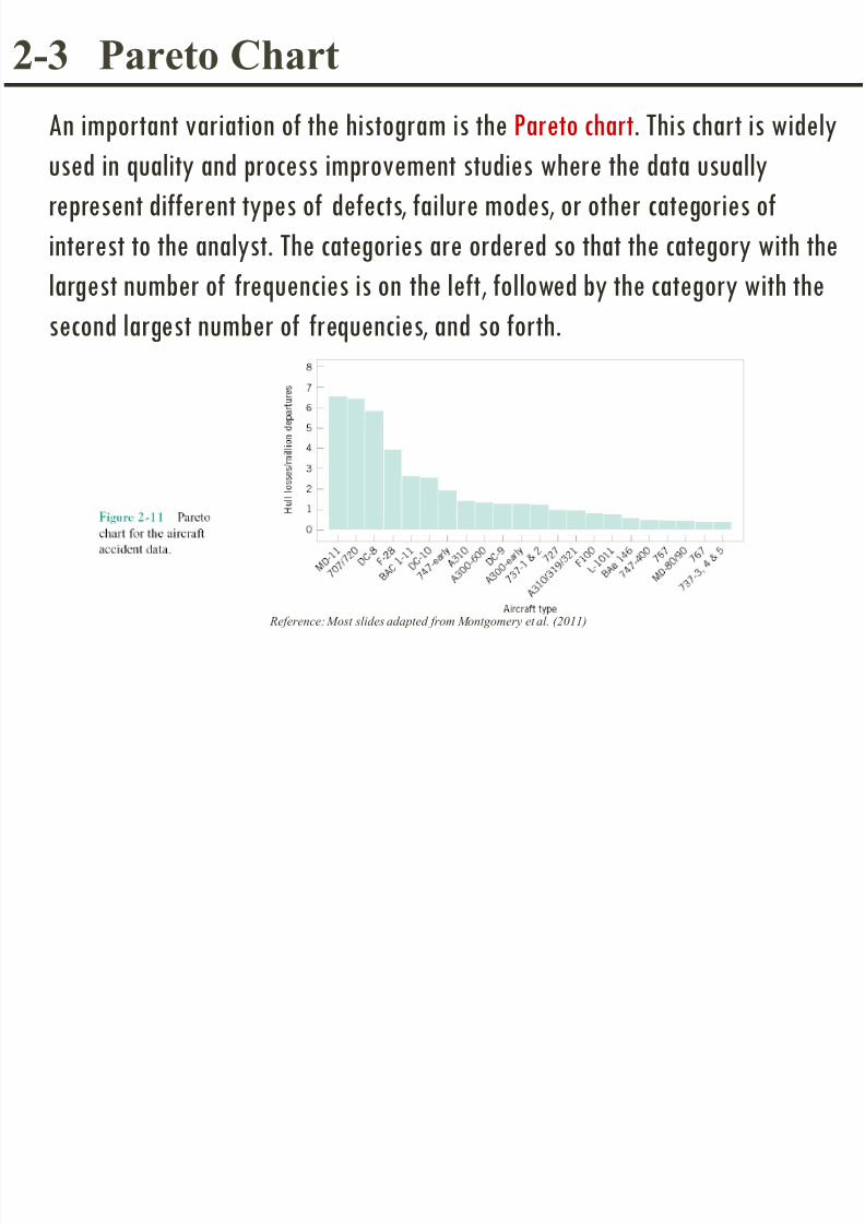
2-3 Pareto Chart

An important variation of the histogram is the Pareto chart. This chart is widely

used in quality and process improvement studies where the data usually

represent different types of defects, failure modes, or other categories of

interest to the analyst. The categories are ordered so that the category with the

largest number of frequencies is on the left, followed by the category with the

second largest number of frequencies, and so forth.




2-4 Box Plots




2-4 Box Plots

0

10

20

30

0 1 2 3 4 5 6 7 9ININ 4998 Credi ts

TOTALSEMESTERS

BOX PLOT EXAMPLE




2-6 Multivariate Data

• The dot diagram, stem-and-leaf diagram, histogram,and box plot are descriptive displays for univariate

data; that is, they convey descriptive information about

a single variable.

•Many engineering problems involve collecting andanalyzing multivariate data, or data on several

different variables.

•In engineering studies involving multivariate data, often

the objective is to determine the relationships among the

variables or to build an empirical model.





Sample Correlation Coefficient




INTERACTIVE EXAMPLEData from an observational study on a Semiconductor Manufacturing environment.

Finished Product: wire bonded to a frame

Measure of Interest (response variable): Pull Strength

Variables: Wire Length and Die Height




DATA SUMMARY AND PRESENTATION INMINITAB

1. Descriptive Statistics: Stat > Basic Statistics > DisplayDescriptive Statistics

2. Dot Plot: Graph > Dotplot

3. Stem and Leaf Plot: Graph > Stem-and-Leaf Plot

4. Histogram: Graph > Histogram To change number of bins: on graph double-click > Binning)

5. *Pareto Chart: Stat > Quality Tools > Pareto Chart

6. Box Plots: Graph > Boxplot

7. All-In-One: Stat > Basic Statistics > Display GraphicalSummary

8. Multivariate Data (Plots and Correlation): Scatter Plots: Graph > Scatterplot; Graph > Matrix Plot;

Correlation: Stat > Basic Statistics > Correlation




DATA SUMMARY AND PRESENTATION IN R

1. Descriptive Statistics: mean(datafile), var(datafile), sd(datafile)

2. *Dot Plot: dotchart(datafile)

3. Stem and Leaf Plot: stem(datafile)

4. Histogram: hist(datafile)

5. Pareto Chart: pareto.chart {qcc}: pareto.chart(defect, ylab = "freq")

6. Box Plots:boxplot(datafile)

7. Multivariate Data (Plots and Correlation): Scatter Plots: plot(datafile)

Correlation: cor(datafile)




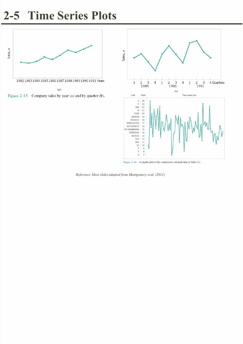
2-5 Time Series Plots

•

A time series or time sequence is a data set in which theobservations are recorded in the order in which they occur.

• A time series plot is a graph in which the vertical axis denotes the

observed value of the variable (say x ) and the horizontal axis denotes

the time (which could be minutes, days, years, etc.).• When measurements are plotted as a time series, we often see

•trends,

•cycles, or

•other broad features of the data




2-5 Time Series Plots



Reference: Most slides adapted from Montgomery et al (2011)

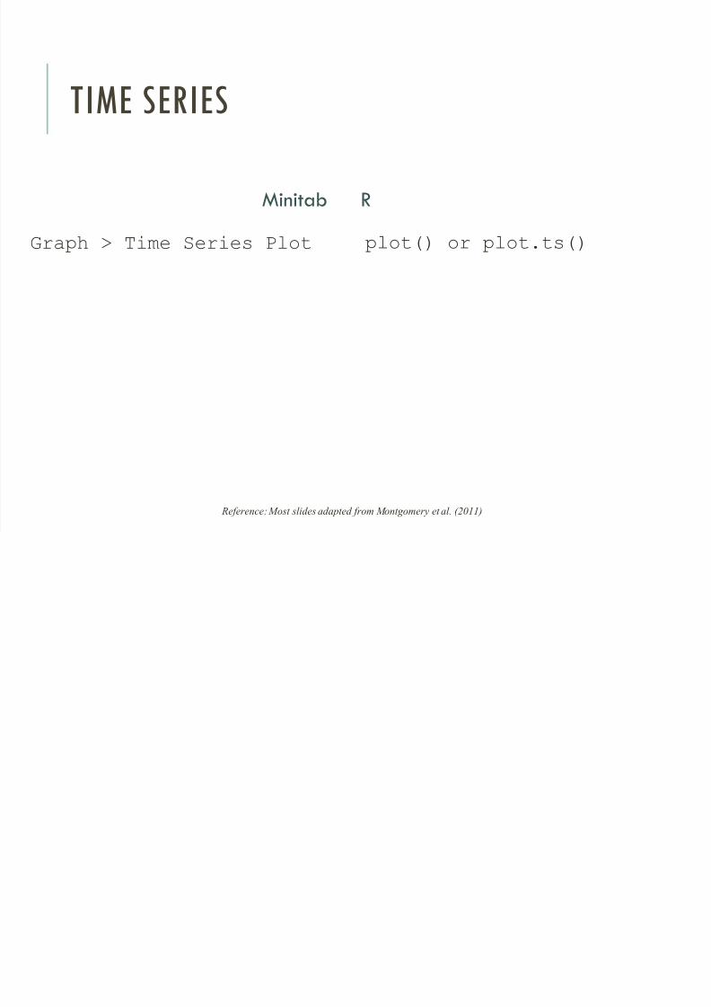
TIME SERIES

Minitab

Graph > Time Series Plot

R

plot() or plot.ts()

Ch2_DataSummaryPresentation_torresgarcia.pdf

Documents

Transcript of Ch2_DataSummaryPresentation_torresgarcia.pdf