Bayesian non-parametrics for time-varying volatility models · prota,˛ kai norisi priimti...
131
TESIS DOCTORAL Bayesian Non-Parametrics for Time- Varying Volatility Models Autor: Audronė Virbickaitė Directores: Concepción Ausín y Pedro Galeano DEPARTAMENTO DE ESTADÍSTICA Getafe, diciembre de 2014
Transcript of Bayesian non-parametrics for time-varying volatility models · prota,˛ kai norisi priimti...

TESIS DOCTORAL
Bayesian Non-Parametrics for Time-Varying Volatility Models
Autor:
Audronė Virbickaitė
Directores:
Concepción Ausín y Pedro Galeano
DEPARTAMENTO DE ESTADÍSTICA
Getafe, diciembre de 2014

TESIS DOCTORAL
BAYESIAN NON-PARAMETRICS FOR TIME-VARYING VOLATILITY MODELS
Autor: Audronė Virbickaitė
Directores: Concepción Ausín y Pedro Galeano
Firma del Tribunal Calificador:
Firma
Presidente: Michael P. Wiper
Vocal: Roberto Casarin
Secretario: M. Pilar Muñoz
Calificación:
Getafe, de de


UNIVERSIDAD CARLOS III DE MADRID
DOCTORAL THESIS
Bayesian Non-Parametrics for Time-VaryingVolatility Models
Author:Audrone Virbickaite
Supervisors:Dr. Concepción Ausín
Dr. Pedro Galeano
A thesis submitted in fulfillment of the requirementsfor the degree of Doctor of Philosophy
in the
Business Administration and Quantitative MethodsStatistics Department
December 2014

Acknowledgements
I want to express my deepest appreciation to a multitude of people who have been a
big part of my life for the last three years during which this thesis came to life. For
professional and personal reasons. For being my mentors and friends. For sharing an
office and traveling with me. For giving advice or just listening. For being from all over
the world.
First of all, I am very grateful to my thesis advisors Conchi and Pedro. Thank you very
much for always finding time for me, for having the patience to teach and let me learn.
And most of all for the academic guidance: Conchi for being an excellent Bayesian and
Pedro for your methodical and attentive approach; after all, the devil is in the detail.
I am especially grateful to Prof. Hedibert Lopes for accepting me as a visiting PhD
student at University of Chicago. I feel extremely lucky to have been able to work with
and learn from such an extraordinary individual and an excellent researcher. Muito
obrigada e espero vê-lo em breve.
Esu labai dekinga savo šeimai Lietuvoje už tai, kad grižus visada jauciuosi namuose.
Aciu mamytei už cepelinus, džiovintus grybus kaskart, kai aplankau, ir už besalygine
meile visada. Aciu tetei ir Vladai už palaikyma, pilnus šaldytuvus alaus, pirti ir šalta
prota, kai norisi priimti karštakoši sprendima. Aciu Jonytei ir Domukui, Jolitukui ir
Andriui ne tik už broliška/seseriška meile, bet ir draugyste. Aciu seneliui Juozui už
meile mokslui ir už buvima pirmu mano pažintu akademiku. Aciu Irutelei už beribe
meile ir dosnuma. Aciu seneliui Jonui, mociutei Jadvygai.
Lo más importante, muchas gracias a Juanín. No solo por acompañarme todos estos
años como mi mejor amigo y familia, pero también por aguantarme en las últimas eta-
pas de la tesis. Gracias por compartir conmigo tu amor a viajar, a historia y a Asturias.
También muchas gracias a mi familia política. Gracias a Pilarita, Rodrigo, Chiqui, Mela,
Alfredo, R7, Lurditas y Pepe por adoptarme y por cuidarme. Por los findes de descanso,
playa de Vidiago y sidra sin fin.
iii

iv
Aciu mano draugams iš Lietuvos ne tik už palaikyma, bet ir už smagiai praleistas poil-
sio minutes, dienas, savaites. Aciu Rutai už nuolatini you can do it! ir už buvima mano
bff, Miglutei, Ingai ir Dovilei už be galo smagius susitikimus. Aciu visai Labanoro kom-
panijai: Gabrieliui, Agnytei, Tomui, Ramintai, Laimuciui, Gabijai, ir dar karta Jonytei
ir Domukui.
Finalmente, quiero agradecer a todos mis compañeros y amigos de la Universidad Car-
los III, el lugar donde durante los últimos cinco años pasé más tiempo que en casa.
Muchas gracias a Juanmi por ayudarme en la resolución de dudas, profesionales o per-
sonales, y por el fondo musical. Pau y Ana, mis hermanitas mayores, las primeras
personas que vi pasar por la tesis y aprendí mucho de ellas. Mil gracias al resto de mis
compañeros con quienes los cinco años en Madrid han sido increíbles: Juliana, Diego,
Carlo-Charly, Mahmoud, Guille, Huro, Diana, Adolfo, Xiuping. Lo siento mucho si
se me olvidó incluir a alguien, sin embargo todos formáis una parte importante de mi
vida.

Contents
Acknowledgements iii
Contents v
List of Figures vii
List of Tables ix
1 Introduction 1
2 Bayesian Inference for Time-Varying Volatility Models 5
2.1 Univariate and multivariate GARCH . . . . . . . . . . . . . . . . . . . . . 6
2.2 Univariate and multivariate SV . . . . . . . . . . . . . . . . . . . . . . . . 22
2.3 Dirichlet Process Mixture . . . . . . . . . . . . . . . . . . . . . . . . . . . 28
2.3.1 Volatility modeling using DPM . . . . . . . . . . . . . . . . . . . . 31
2.4 Sequential Monte Carlo . . . . . . . . . . . . . . . . . . . . . . . . . . . . 33
2.5 Conclusions . . . . . . . . . . . . . . . . . . . . . . . . . . . . . . . . . . . 36
3 A Bayesian Approach to the ADCC Model with Application to Portfolio Se-
lection 39
3.1 Model, inference and prediction . . . . . . . . . . . . . . . . . . . . . . . . 42
3.1.1 The Bayesian non-parametric ADCC model . . . . . . . . . . . . 42
3.1.2 MCMC algorithm . . . . . . . . . . . . . . . . . . . . . . . . . . . . 46
3.1.3 Prediction . . . . . . . . . . . . . . . . . . . . . . . . . . . . . . . . 49
3.2 Portfolio decisions . . . . . . . . . . . . . . . . . . . . . . . . . . . . . . . 51
3.3 Simulation study . . . . . . . . . . . . . . . . . . . . . . . . . . . . . . . . 53
3.4 Real data and results . . . . . . . . . . . . . . . . . . . . . . . . . . . . . . 55
3.4.1 Estimation . . . . . . . . . . . . . . . . . . . . . . . . . . . . . . . . 56
3.4.2 Portfolio allocation . . . . . . . . . . . . . . . . . . . . . . . . . . . 64
v
Contents vi
3.5 Conclusions . . . . . . . . . . . . . . . . . . . . . . . . . . . . . . . . . . . 68
4 A Bayesian Non-Parametric Approach to a MSSV Model with Particle Learn-
ing 69
4.1 SV-DPM Model . . . . . . . . . . . . . . . . . . . . . . . . . . . . . . . . . 71
4.1.1 MCMC for SV-DPM . . . . . . . . . . . . . . . . . . . . . . . . . . 74
4.1.2 PL for SV-DPM . . . . . . . . . . . . . . . . . . . . . . . . . . . . . 75
4.1.3 Simulation exercise . . . . . . . . . . . . . . . . . . . . . . . . . . . 76
4.2 MSSV-DPM Model . . . . . . . . . . . . . . . . . . . . . . . . . . . . . . . 80
4.2.1 PL for MSSV-DPM . . . . . . . . . . . . . . . . . . . . . . . . . . . 82
4.2.2 Simulated data . . . . . . . . . . . . . . . . . . . . . . . . . . . . . 85
4.3 Real data application . . . . . . . . . . . . . . . . . . . . . . . . . . . . . . 87
4.4 Discussion . . . . . . . . . . . . . . . . . . . . . . . . . . . . . . . . . . . . 95
5 Conclusions and Extensions 97
5.1 Conclusions . . . . . . . . . . . . . . . . . . . . . . . . . . . . . . . . . . . 97
5.2 Extensions . . . . . . . . . . . . . . . . . . . . . . . . . . . . . . . . . . . . 98
Bibliography 101

List of Figures
3.1 Contour plots of the true and estimated one-step-ahead predictive den-
sities, f (rT+1 | rT), for the three simulated data sets. . . . . . . . . . . . . 54
3.2 Densities of the elements of the one-step-ahead covariance matrices for
Normal and Student-t data estimated using (a) DPM and Normal and
(b) DPM and Student-t errors. . . . . . . . . . . . . . . . . . . . . . . . . . 57
3.3 Log-returns (in %) and histograms of Apple Inc. and NASDAQ Ind. index. 57
3.4 Traces, histograms and running mean plots of A = c/(1 + c) for fully
symmetric BNP-DCC (M0) and asymmetric BNP-ADCC (M1) models. . 59
3.5 Contours of the predictive densities for rT+1 for fully symmetric BNP-
DCC (M0) and asymmetric BNP-ADCC (M1) models. . . . . . . . . . . . 60
3.6 Marginal log-predictive densities for the one-step-ahead Apple Inc. (r(1)T+1)
and NASDAQ Ind. (r(2)T+1) return data, for fully symmetric BNP-DCC
(M0) and asymmetric BNP-ADCC (M1) models. . . . . . . . . . . . . . . 60
3.7 Log-returns (in %) of Apple Inc. and NASDAQ Ind. index for t = 3099, . . . , 3331. 61
3.8 Posterior distributions of one-step-ahead volatilities for fully symmetric
BNP-DCC (M0) and asymmetric BNP-ADCC (M1) models. . . . . . . . . 62
3.9 Posterior distributions for A = c/(1 + c) and a number of non-empty
clusters z? for different hyper-parameters for c ∼ G(a0, b0) for BNP-
ADCC model for Apple-NASDAQ data. . . . . . . . . . . . . . . . . . . . 63
3.10 Prior and posterior distributions for c for BNP-ADCC model for Apple-
NASDAQ data. . . . . . . . . . . . . . . . . . . . . . . . . . . . . . . . . . 64
3.11 Posterior distributions of one-step-ahead optimal portfolio weights p?T+1
and overall portfolio variances σ2?T+1 for fully symmetric BNP-DCC (M0)
and asymmetric BNP-ADCC (M1) models . . . . . . . . . . . . . . . . . . 65
3.12 A sequence of portfolio weights and their corresponding 95% CIs for
τ = 1, . . . , 233 for fully symmetric BNP-DCC (M0) and asymmetric BNP-
ADCC (M1) models. . . . . . . . . . . . . . . . . . . . . . . . . . . . . . . 66
3.13 A sequence of portfolio variances and their corresponding 95% CIs for
τ = 1, . . . , 233 for fully symmetric BNP-DCC (M0) and asymmetric BNP-
ADCC (M1) models. . . . . . . . . . . . . . . . . . . . . . . . . . . . . . . 66
vii

List of Figures viii
3.14 Mean cumsum of the of 95% CI width for the optimal portfolio weights
and variances for τ = 1, . . . , 233 for fully symmetric BNP-DCC (M0) and
asymmetric BNP-ADCC (M1) models. . . . . . . . . . . . . . . . . . . . . 67
4.1 Density of a mixture of 7 Normals and the density of the simulated data
compared to the predictive density for εt = log ε2t , estimated by PL and
MCMC for T = 3000. . . . . . . . . . . . . . . . . . . . . . . . . . . . . . . 78
4.2 Posterior distributions of the log-volatilities for MCMC and PL for T =
1000, 2000 and 3000. . . . . . . . . . . . . . . . . . . . . . . . . . . . . . . . 79
4.3 PL parameter estimates with 95% CI for one run of 300k particles, com-
pared to the true parameter values. . . . . . . . . . . . . . . . . . . . . . . 79
4.4 Simulated data: daily returns (top graph), true and estimated log-volatilities
(middle graph) and true and estimated regimes (bottom graph). . . . . . 85
4.5 Simulated data: true and estimated density for log-squared return dis-
tribution. . . . . . . . . . . . . . . . . . . . . . . . . . . . . . . . . . . . . . 86
4.6 Simulated data: true and estimated parameters with 95% HPD intervals. 86
4.7 Simulated data II: daily returns (top graph), true and estimated volatili-
ties (middle graph) and true and estimated regimes (bottom graph). . . 87
4.8 Daily log-returns (in %) and corresponding histograms for S&P500, Ford
and Natural gas data. . . . . . . . . . . . . . . . . . . . . . . . . . . . . . . 88
4.9 Estimated densities for the log-squared error term for SV-DPM and MSSV-
DPM models. . . . . . . . . . . . . . . . . . . . . . . . . . . . . . . . . . . 90
4.10 Filtered volatilities and volatility states for S&P500 data for SV-DPM and
MSSV-DPM models. . . . . . . . . . . . . . . . . . . . . . . . . . . . . . . 91
4.11 Filtered volatilities and volatility states for Ford data for SV-DPM and
MSSV-DPM models. . . . . . . . . . . . . . . . . . . . . . . . . . . . . . . 93
4.12 Filtered volatilities and volatility states for Gas data for SV-DPM and
MSSV-DPM models. . . . . . . . . . . . . . . . . . . . . . . . . . . . . . . 94

List of Tables
3.1 Posterior means, medians and 95% credible intervals for the number of
non-empty clusters z?, concentration parameter c, quantity A = c/(1 +
c), and model parameters for the three simulated data sets. . . . . . . . . 56
3.2 Descriptive statistics of the Apple Inc. and NASDAQ Ind. index return
series. . . . . . . . . . . . . . . . . . . . . . . . . . . . . . . . . . . . . . . . 58
3.3 Estimation results for Apple Inc. (1) and NASDAQ Ind. (2) returns as-
suming fully symmetric (M0) and asymmetric (M1) multivariate GARCH
models. . . . . . . . . . . . . . . . . . . . . . . . . . . . . . . . . . . . . . . 59
3.4 Cumulative log-predictive likelihoods for fully symmetric BNP-DCC (M0)
and asymmetric BNP-ADCC (M1) models. . . . . . . . . . . . . . . . . . 62
3.5 Posterior means, medians and confidence intervals for the elements of
the one-step-ahead volatility matrix for fully symmetric BNP-DCC (M0)
and asymmetric BNP-ADCC (M1) models. . . . . . . . . . . . . . . . . . 63
3.6 Posterior means and 95% credible intervals for A = c/(1 + c) and a
number of non-empty clusters z? for different hyper-parameters for c ∼G(a0, b0) for BNP-ADCC model for Apple-NASDAQ data. . . . . . . . . 63
3.7 Posterior mean, median and 95% credible intervals for the optimal one-
step-ahead portfolio weight and variance. . . . . . . . . . . . . . . . . . . 64
4.1 CPU time in seconds for MCMC and PL. . . . . . . . . . . . . . . . . . . . 77
4.2 Parameter estimates and their corresponding 95% CIs for PL and MCMC
for T = 1000, 2000, 3000. . . . . . . . . . . . . . . . . . . . . . . . . . . . . 78
4.3 Descriptive statistics for S&P500, Ford and Gas data. . . . . . . . . . . . . 88
4.4 Parameter estimation for SV-DPM and MSSV-DPM models for S&P500
data at time T. . . . . . . . . . . . . . . . . . . . . . . . . . . . . . . . . . . 90
4.5 LPS and LPTSα for SV-DPM and MSSV-DPM for S&P500 data. . . . . . . 92
4.6 Parameter estimation for SV-DPM and MSSV-DPM models for Ford data
at time T. . . . . . . . . . . . . . . . . . . . . . . . . . . . . . . . . . . . . . 92
4.7 LPS and LPTSα for SV-DPM and MSSV-DPM for Ford data. . . . . . . . . 93
ix

List of Tables x
4.8 Parameter estimation for SV-DPM and MSSV-DPM models for Gas data
at time T. . . . . . . . . . . . . . . . . . . . . . . . . . . . . . . . . . . . . . 95
4.9 LPS and LPTSα for SV-DPM and MSSV-DPM for Gas data. . . . . . . . . 95

Skirta mano šeimai ir Juanui.
xi

Chapter 1
Introduction
Understanding, modeling and predicting volatilities of financial time series has been
extensively researched for more than 30 years and the interest in the subject is far
from decreasing. Volatility prediction has a very wide range of applications in fi-
nance, for example, in portfolio optimization, risk management, asset allocation, as-
set pricing, etc. The two most popular approaches to model volatility are based on
the Autoregressive Conditional Heteroscedasticity (ARCH) type and Stochastic Volati-
lity (SV) type models. The seminal paper of Engle (1982) proposed the initial ARCH
model while Bollerslev (1986) generalized the purely autoregressive ARCH into an
ARMA-type model, called the Generalized Autoregressive Conditional Heteroscedas-
ticity (GARCH) model. On the other hand, Taylor (1982, 1986) proposed to model the
volatility as an unobserved process, giving the start to SV models. Since then, there
has been a very large amount of research on the topic, stretching to various model
extensions and generalizations. The supply of models, univariate and multivariate,
GARCH and SV, has been growing over the years. Meanwhile, the researchers have
been addressing two important topics: looking for the best specification for the errors
and selecting the most efficient approach for inference and prediction. This thesis puts
emphasis on these two questions as well.
Besides selecting the best model for the volatility, distributional assumptions for the
returns are equally important. It is well known, that every prediction, in order to be
useful, has to come with a certain precision measurement. In this way the agent can
1
Chapter 1. Introduction 2
know the risk she is facing, i.e. uncertainty. Distributional assumptions permit to quan-
tify this uncertainty about the future. Traditionally, the errors have been assumed to be
Gaussian, however, it has been widely acknowledged that financial returns display fat
tails and are not conditionally Normal. Therefore, it is common to assume a Student-t
distribution, see Bollerslev (1987), He & Teräsvirta (1999), Bai et al. (2003) and Jacquier
et al. (2004), among many others. However, the assumption of Gaussian or Student-t
distributions is rather restrictive. An alternative approach is to use a mixture of distri-
butions, which can approximate arbitrarily any distribution given a sufficient number
of mixture components. A mixture of two Normals was used by Bai et al. (2003), Ausín
& Galeano (2007) and Giannikis et al. (2008), among others. These authors have shown
that the models with the mixture distribution for the errors outperformed the Gaussian
ones and do not require additional restrictions on the degrees of freedom parameter as
the Student-t one.
As for the inference and prediction, the Bayesian approach is especially well-suited
for GARCH and SV models and provides some advantages compared to classical esti-
mation techniques, as outlined by Ardia & Hoogerheide (2010). Firstly, the positivity
constraints on the parameters to ensure positive variance, may encumber some op-
timization procedures. In the Bayesian setting, constraints on the model parameters
can be incorporated via priors. Secondly, in most of the cases we are more interested
not in the model parameters directly, but in some non-linear functions of them. In the
maximum likelihood (ML) setting, it is quite troublesome to perform inference on such
quantities, while in the Bayesian setting it is usually straightforward to obtain the pos-
terior distribution of any non-linear function of the model parameters. Furthermore,
in the classical approach, models are usually compared by any other means than the
likelihood. In the Bayesian setting, marginal likelihoods and Bayes factors allow for
consistent comparison of non-nested models while incorporating Occam’s razor for
parsimony. Also, Bayesian estimation provides reliable results even for finite samples.
Finally, Hall & Yao (2003) add that the ML approach presents some limitations when
the errors are heavy tailed, also the convergence rate is slow and the estimators may
not be asymptotically Gaussian.
Therefore in this thesis we consider different Bayesian non-parametric specifications
for the errors for GARCH and SV models. Also, we employ two Bayesian estimation
approaches: Markov Chain Monte Carlo (MCMC) and Sequential Monte Carlo (SMC).
Chapter 1. Introduction 3
The thesis is structured as follows:
Chapter 2 reviews the existing literature on the most relevant Bayesian inference meth-
ods for univariate and multivariate GARCH and SV models. The advantages and
drawbacks of each procedure are outlined as well as the advantages of the Bayesian
approach versus classical procedures. The chapter makes emphasis on Bayesian non-
parametrics for time-varying volatility models that avoid imposing arbitrary paramet-
ric distributional assumptions. Finally, the chapter presents an alternative Bayesian
estimation technique - Sequential Monte Carlo, that allows for an on-line type infer-
ence. The major part of the contents of this chapter resulted into a paper by Virbickaite
et al. (2013), which has been accepted in the Journal of Economic Surveys.
Chapter 3 considers an asymmetric dynamic conditional correlation (ADCC) model to
estimate the time-varying correlations of financial returns where the individual vola-
tilities are driven by GJR-GARCH models. This composite model takes into consider-
ation the asymmetries in individual assets’ volatilities, as well as in the correlations.
The errors are modeled using a Dirichlet location-scale mixture of multivariate Nor-
mals allowing for a flexible return distribution in terms of skewness and kurtosis. This
gives rise to a Bayesian non-parametric ADCC (BNP-ADCC) model, as opposed to a
symmetric specification, called BNP-DCC. Then these two models are estimated using
MCMC and compared by considering a sample of Apple Inc. and NASDAQ Industrial
index daily returns. The obtained results reveal that for this particular data set the
BNP-ADCC outperforms the BNP-DCC model. Finally, an illustrative asset allocation
exercise is presented. The contents of this chapter resulted into a paper by Virbickaite,
Ausín & Galeano (2014), which has been accepted in Computational Statistics and Data
Analysis.
Chapter 4 designs a Particle Learning (PL) algorithm for estimation of Bayesian non-
parametric Stochastic Volatility models for financial data. The performance of this par-
ticle method is then compared with the standard MCMC methods for non-parametric
SV models. PL performs as well as MCMC, and at the same time allows for on-line
type inference. The posterior distributions are updated as new data is observed, which
is prohibitively costly using MCMC. Further, a new non-parametric SV model is pro-
posed that incorporates Markov switching jumps. The proposed model is estimated

Chapter 1. Introduction 4
by using PL and tested on simulated data. Finally, the performance of the two non-
parametric SV models, with and without Markov switching, is compared by using real
financial time series. The results show that including a Markov switching specification
provides higher predictive power in the tails of the distribution. The contents of this
chapter resulted into a working paper by Virbickaite, Lopes, Ausín & Galeano (2014).
Finally, Chapter 5 concludes and proposes general future research lines that could be
viewed as natural extensions of the ideas presented in the thesis.

Chapter 2
Bayesian Inference for Time-Varying
Volatility Models
This chapter reviews the existing Bayesian inference methods for univariate and mul-
tivariate GARCH and SV models while having in mind their error specifications. The
main emphasis of this chapter is on the recent development of an alternative inference
approach for these models using Bayesian non-parametrics. The classical paramet-
ric modeling, relying on a finite number of parameters, although so widely used, has
some certain drawbacks. Since the number of parameters for any model is fixed, one
can encounter underfitting or overfitting, which arises from the misfit between the data
available and the parameters needed to estimate. Then, in order to avoid assuming
wrong parametric distributions, which may lead to inconsistent estimators, it is better
to consider a semi- or non-parametric approach. Bayesian non-parametrics may lead
to less constrained models than classical parametric Bayesian statistics and provide an
adequate description of the data, especially when the conditional return distribution is
far away from Gaussian.
The literature on non-parametric GARCH and SV type models is still very recent, how-
ever, the popularity of the topic is rapidly increasing, see Jensen & Maheu (2010, 2013,
2014), Delatola & Griffin (2011, 2013) and Ausín et al. (2014). All of them have consid-
ered infinite mixtures of Gaussian distributions with a Dirichlet process (DP) prior over
the mixing distribution, which results into DP mixture (DPM) models (see Lo 1984 and
Ferguson 1973, among others). This approach proves to be the most popular Bayesian
5

Chapter 2. Review 6
non-parametric modeling procedure so far. The results over the papers have been con-
sistent: Bayesian non-parametric methods lead to more flexible models and are better
in explaining heavy-tailed return distributions, which parametric models cannot fully
capture.
The outline of this chapter is as follows. Sections 2.1 and 2.2 shortly introduce univari-
ate and multivariate GARCH and SV models and different inference and prediction
methods. Section 2.3 introduces the Bayesian non-parametric modeling approach and
reviews the limited literature of this area in time-varying volatility models. Finally,
Section 2.5 concludes.
2.1 Univariate and multivariate GARCH
In this section we shortly introduce the most popular univariate and multivariate
GARCH specifications. In the description of the models and the review of the inference
methods we are not going to enter into the technical details of the Bayesian algorithms
and refer to Robert & Casella (2004) for a more detailed description of the mentioned
Bayesian techniques.
Univariate GARCH
The general structure of an asset return series modeled by a GARCH-type models can
be written as:
rt = µt + at = µt +√
htεt, (2.1)
where µt = E[rt|I t−1] is the conditional mean given I t−1, the information up to time
t− 1, at is the mean corrected returns of the asset at time t, ht = Var[rt|I t−1] is the
conditional variance given I t−1 and εt is the standard white noise shock. There are
several ways to model the conditional mean µt. The usual assumptions are to consider
that the mean is either zero, equal to a constant (µt = µ), or follows an ARMA(p,q) pro-
cess. However, sometimes the mean is also modeled as a function of the variance, say
g(ht), which leads to the GARCH-in-Mean models. On the other hand, the conditional
Chapter 2. Review 7
variance, ht, is usually modeled using the GARCH-family models. In the basic GARCH
model the conditional volatility of the returns depends on a sum of three parts: a con-
stant variance as the long-run average, a linear combination of the past conditional
volatilities and a linear combination of the past mean squared returns. For instance, in
the GARCH(1,1) model, the conditional variance at time t is given by
ht = ω + αa2t−1 + βht−1, for t = 1, . . . , T. (2.2)
There are some restrictions which have to be imposed such as ω > 0, α, β ≥ 0 for posi-
tive variance, and α + β < 1 for covariance stationarity.
Nelson (1991) proposed the exponential GARCH (EGARCH) model that acknowledges
the existence of asymmetry in the volatility response to the changes in the returns,
sometimes also called “leverage effect", introduced by Black (1976). Negative shocks
to the returns have a stronger effect on volatility than positive ones. Other ARCH ex-
tensions that try to incorporate the leverage effect are the GJR model by Glosten et al.
(1993) and the TGARCH of Zakoian (1994), among many others. As Engle (2004) puts it,
“there is now an alphabet soup” of ARCH family models, such as AARCH, APARCH,
FIGARCH, STARCH etc, which try to incorporate such return features as fat tails, vola-
tility clustering and volatility asymmetry. Papers by Bollerslev et al. (1992), Bollerslev
et al. (1994), Engle (2002b), Ishida & Engle (2002) provide extensive reviews of the ex-
isting ARCH-type models. Bera & Higgins (1993) review ARCH type models, discuss
their extensions, estimation and testing, also numerous applications. Additionally, one
can find an explicit review with examples and applications concerning GARCH-family
models in Tsay (2010) and Chapter 1 in Teräsvirta (2009).
The most used estimation approach for GARCH-family models is the maximum likeli-
hood method. However, recently there has been a rapid development of Bayesian esti-
mation techniques, which offer some advantages compared to the frequentist approach
as already discussed in the beginning of this chapter. In addition, in the empirical fi-
nance setting, the frequentist approach presents an uncertainty problem. For instance,
optimal allocation is greatly affected by the parameter uncertainty, which has been rec-
ognized in a number of papers, see Jorion (1986) and Greyserman et al. (2006), among
others. These authors conclude that in the frequentist setting the estimated parameter
values are considered to be the true ones, therefore, the optimal portfolio weights tend

Chapter 2. Review 8
to inherit this estimation error. However, instead of solving the optimization prob-
lem on the basis of the choice of unique parameter values, the investor can choose
the Bayesian approach, because it accounts for parameter uncertainty, as seen in Kang
(2011) and Jacquier & Polson (2013), for example. A number of papers in this field
have explored different Bayesian procedures for inference and prediction and differ-
ent approaches to model the fat-tailed errors and/or asymmetric volatility. The recent
development of modern Bayesian computational methods, based on Monte Carlo ap-
proximations and MCMC methods have facilitated the usage of Bayesian techniques,
see e.g. Robert & Casella (2004).
The standard Gibbs sampling procedure does not make the list because it cannot be
used due to the recursive nature of the conditional variance: the conditional posterior
distributions of the model parameters are not of a simple form. One of the alternatives
is the Griddy-Gibbs sampler as in Bauwens & Lubrano (1998). They discuss that previ-
ously used importance sampling and Metropolis algorithms have certain drawbacks,
such as that they require a careful choice of a good approximation of the posterior den-
sity. The authors propose a Griddy-Gibbs sampler which explores analytical properties
of the posterior density as much as possible. In their paper GARCH model has Student-
t errors, which allows for fat tails. The authors choose to use flat (Uniform) priors on
parameters (ω, α, β) with whatever region is needed to ensure the positivity of vari-
ance, however, the flat prior for the degrees of freedom cannot be used, because then
the posterior density is not integrable. Instead, they choose a half-right side of Cauchy.
The posteriors of the parameters were found to be skewed, which is a disadvantage
for the commonly used Gaussian approximation. On the other hand, Ausín & Galeano
(2007) modeled the errors of a GARCH model with a mixture of two Gaussian distri-
butions. The advantage of this approach, compared to that of Student-t errors, is that
if the number of the degrees of freedom is very small (less than 5), some moments may
not exist. The authors have chosen flat priors for all the parameters, and discovered
that there is little sensitivity to the change in the prior distributions (from Uniform to
Beta), unlike in Bauwens & Lubrano (1998), where the sensitivity for the prior choice
for the degrees of freedom is high. Other articles using a Griddy-Gibbs sampling ap-
proach include Bauwens & Lubrano (2002), who have modeled asymmetric volatility
with Gaussian innovations and have used Uniform priors for all the parameters, and
by Wago (2004), who explored an asymmetric GARCH model with Student-t errors.
Chapter 2. Review 9
Another MCMC algorithm used in estimating GARCH model parameters, is the
Metropolis - Hastings (MH) method, which samples from a candidate density and then
accepts or rejects the draws depending on a certain acceptance probability. Ardia (2006)
modeled the errors as Gaussian distributed with zero mean and unit variance while
the priors are chosen as Gaussian and a MH algorithm is used to draw samples from
the joint posterior distribution. The author has carried out a comparative analysis be-
tween ML and Bayesian approaches, finding, as in other papers, that some posterior
distributions of the parameters were skewed, thus warning against the abusive use of
the Gaussian approximation. Also, Ardia (2006) has performed a sensitivity analysis
of the prior means and scale parameters and concluded that the initial priors in this
case are vague enough. This approach has been also used by Müller & Pole (1998),
Nakatsuma (2000) and Vrontos et al. (2000), among others. A special case of the MH
method is the random walk Metropolis-Hastings (RWMH) where the proposal draws
are generated by randomly perturbing the current value using a spherically symmetric
distribution. A usual choice is to generate candidate values from a Gaussian distribu-
tion where the mean is the previous value of the parameter and the variance can be
calibrated to achieve the desired acceptance probability. This procedure is repeated at
each MCMC iteration. Ausín & Galeano (2007) have also carried out a comparison of
estimation approaches, Griddy-Gibbs, RWMH and ML. Apparently, RWMH has dif-
ficulties in exploring the tails of the posterior distributions and ML estimates may be
rather different for those parameters where posterior distributions are skewed.
In order to select one of the algorithms, one might consider some criteria, such as fast
convergence for example. Asai (2006) numerically compares some of these approaches
in the context of GARCH models. The Griddy-Gibbs method is capable in handling the
shape of the posterior by using shorter MCMC chains comparing with other methods,
also, it is flexible regarding parametric specification of the model. However, it can re-
quire a lot of computational time. This author also investigates MH, adaptive rejection
Metropolis sampling (ARMS), proposed by Gilks et al. (1995), and acceptance-rejection
MH algorithms (ARMH), proposed by Tierney (1994). For more in detail about each
method in GARCH models see Nakatsuma (2000) and Kim et al. (1998), among others.
Using simulated data, Asai (2006) calculated geometric averages of inefficiency factors
for each method. Inefficiency factor is just an inverse of Geweke (1992) efficiency fac-
tor. According to this, the ARMH algorithm performed the best. Also, computational
Chapter 2. Review 10
time was taken into consideration, where ARMH clearly outperformed MH and ARMS,
while Griddy-Gibbs stayed just a bit behind. The author observes that even though the
ARMH method showed the best results, the posterior densities for each parameter did
not quite explore the tails of the distributions, as desired. In this case Griddy-Gibbs per-
forms better; also, it requires less draws than ARMH. Bauwens & Lubrano (1998) inves-
tigate one more convergence criteria, proposed by Yu & Mykland (1998), which is based
on cumulative sum (cumsum) statistics. It basically shows that if MCMC is converg-
ing, the graph of a certain cumsum statistic against time should approach zero. Their
employed Griddy-Gibbs algorithm converged in all four parameters quite fast. Then,
the authors explored the advantages and disadvantages of alternative approaches: the
importance sampling and the MH algorithm. Considering importance sampling, one
of the main disadvantages, as mentioned before, is to find a good approximation of
the posterior density (importance function). Also, comparing with Griddy-Gibbs al-
gorithm, the importance sampling requires much more draws to get smooth graphs of
the marginal densities. For the MH algorithm, same as in importance sampling, a good
approximation needs to be found. Also, compared to Griddy-Gibbs, the MH algorithm
did not fully explore the tails of the distribution, unless for a very big number of draws.
Another important aspect of the Bayesian approach, as commented before, is the ad-
vantage in model selection compared to classical methods. Miazhynskaia & Dorffner
(2006) reviews some Bayesian model selection methods using MCMC for GARCH-type
models, which allow for the estimation of either marginal model likelihoods, Bayes
factors or posterior model probabilities. These are compared to the classical model se-
lection criteria showing that Bayesian approach clearly considers model complexity in
a more unbiased way. Also, Chen et al. (2009) includes a revision of Bayesian selec-
tion methods for asymmetric GARCH models, such as the GJR-GARCH and threshold
GARCH. They show how using Bayesian approach it is possible to compare complex
and non-nested models to choose for example between GARCH and stochastic vola-
tility models, between symmetric or asymmetric GARCH models or to determine the
number of regimes in threshold processes, among others.
Markov Switching GARCH (MS-GARCH). One of the most prominent features of
the volatilities of financial time series is a very high persistence of the variance process,
which in some cases is very close to having a unit root. Some authors argue that the
Chapter 2. Review 11
upward bias in the persistence parameter might occur due to the presence of struc-
tural changes in volatility, which simple GARCH models do not account for. Therefore,
Hamilton & Susmel (1994) and Cai (1994) independently proposed a Markov Switch-
ing ARCH model, which later was generalized by Gray (1996) into MS-GARCH. Dif-
ferently than simple GARCH model, defined in Equation 2.1 and Equation 2.2, the
MS-GARCH model has the following representation:
rt = µst + at = µst +√
htεt,
ht = ωst + αst a2t−1 + βst ht−1, for t = 1, . . . , T,
where st are the regime variables following a J-state first order Markov Process with
the following transition probabilities:
pij = P [st = j|st−1 = i] , for i, j = 1, . . . , J.
Kaufmann & Frühwirth-Schnatter (2002) designed an MCMC scheme to generate a
sample from the posterior of a MS-ARCH model, which has not been done before,
by combining a multi-move sampling of a hidden Markov process with Metropolis –
Hastings for parameter estimation. The authors have performed model selection us-
ing Bayes factors and model likelihoods to determine the number of states and the
number of autoregressive parameters in the volatility process. Bauwens et al. (2010)
note that ML estimation of MS-GARCH model is basically impossible, because of the
unobservable regimes. Therefore, they propose an MCMC algorithm that evades the
problem of path dependence by treating the state variables as additional parameters.
The authors carry out an extensive simulation study to evaluate the performance of
the algorithm and then apply it to a sample of S&P500 daily returns. Based on the BIC
they find that the MS-GARCH model with two regimes fits the data better than the MS-
ARCH model. Next, Henneke et al. (2011) generalize the MS-GARCH model by includ-
ing the ARMA process in the return evolution, resulting into a MS-ARMA–GARCH
model. The authors design a MCMC scheme for estimation and compare their model
with the one of Hamilton & Susmel (1994) by using the same data set and conclude

Chapter 2. Review 12
that full MS–ARMA–GARCH models outperform models such as of Hamilton & Sus-
mel (1994). Bauwens et al. (2014) design a particle MCMC (PMCMC) method for es-
timation, called particle Gibbs sampler, which samples state variables jointly, rather
than individually, as in Bauwens et al. (2010), and then sample the parameters given
the states. The authors compare the performance of the MS-GARCH model with the
change point GARCH (CP-GARCH), as in He & Maheu (2010), where the chain is not
recurrent, differently than in Markov switching models. Bauwens et al. (2014) intro-
duce an efficient method to compute marginal likelihoods, which was not feasible until
then. The authors apply the two models - MS and CP - to several series of financial re-
turns and find that MS-GARCH models with two regimes dominate CP-GARCH mod-
els. For some other financial returns, more regimes or breaks are necessary. However,
MS-GARCH models are preferable in all cases. Finally, Billio et al. (2014) develop an
efficient MCMC estimation approach for MS-GARCH model, which simultaneously
generates the states from their joint distribution. The authors design a multiple-try
sampling strategy, where a candidate path of the state variable is obtained by applying
FFBS algorithm to an auxiliary MS-GARCH model. Billio et al. (2014) use the same data
set as in Bauwens et al. (2014) and obtained results that are consistent with the ones in
Bauwens et al. (2014).
Multivariate GARCH
Returns and volatilities depend on each other, so multivariate analysis is a more natural
and useful approach. The starting point of multivariate volatility models is a univariate
GARCH, thus the most simple MGARCH models can be viewed as direct generaliza-
tions of their univariate counterparts. Consider a multivariate return series rtTt=1 of
dimension K. Then
rt = µt + at = µt + H1/2t εt,
where µt = E[rt|I t−1], at are mean-corrected returns, εt is a random vector, such
that E[εt] = 0 and Cov[εt] = IK and H1/2t is a positive definite matrix of dimensions
K× K, such that Ht is the conditional covariance matrix of rt, i.e., Cov[rt|I t−1] =
H1/2t Cov[εt](H1/2
t )′ = Ht. There is a wide range of MGARCH models, where most of
them differ in specifying Ht. In the rest of this section we will review the most popular

Chapter 2. Review 13
of them and also the different Bayesian approaches to make inference and prediction.
For general reviews on MGARCH models, see Bauwens et al. (2006), Silvennoinen &
Teräsvirta (2009) and Tsay (2010) (Chapter 10), among others.
Regarding inference, one can also consider the same arguments provided in the uni-
variate GARCH case above. Maximum likelihood estimation for MGARCH models can
be obtained by using numerical optimization algorithms, such as Fisher scoring and
Newton-Raphson. Vrontos et al. (2003b) have estimated several bivariate ARCH and
GARCH models and found that some ML estimates of the parameters were quite dif-
ferent from their Bayesian counterparts. This was due to the non-Normality of the pa-
rameters. Thus, the authors suggest careful interpretation of the classical estimation ap-
proach. Also, Vrontos et al. (2003b) found it difficult to evaluate the classical estimates
under the stationarity conditions, and consequently the resulting parameters, evalu-
ated ignoring the stationarity constraints, produced non-stationary estimates. These
difficulties can be overcome using the Bayesian approach.
VEC, DVEC and BEKK. The VEC model was proposed by Bollerslev et al. (1988),
where every conditional variance and covariance (elements of the Ht matrix) is a func-
tion of all lagged conditional variances and covariances, as well as lagged squared
mean-corrected returns and cross-products of returns. Using this unrestricted VEC for-
mulation, the number of parameters increases dramatically. For example, if K = 3, the
number of parameters to estimate will be 78, and if K = 4, the number of parameters
increases to 210, see Bauwens et al. (2006) for the explicit formula for the number of pa-
rameters in VEC models. To overcome this difficulty, Bollerslev et al. (1988) simplified
the VEC model by proposing a diagonal VEC model:
Ht = Ω + A (at−1a′t−1) + B Ht−1,
where indicates the Hadamard product, Ω, A and B are symmetric K× K matrices.
As noted in Bauwens et al. (2006), Ht is positive definite provided that Ω, A, B and the
initial matrix H0 are positive definite. However, these are quite strong restrictions on
the parameters. Also, DVEC model does not allow for dynamic dependence between
volatility series. In order to avoid such strong restrictions on the parameter matrices,
Engle & Kroner (1995) propose the BEKK model, which is just a special case of VEC and,

Chapter 2. Review 14
consequently, less general. It has the attractive property that the conditional covariance
matrices are positive definite by construction. The model looks as follows:
Ht = Ω∗Ω∗′+ A∗(at−1a′t−1)A∗
′+ B∗Ht−1B∗
′, (2.3)
where Ω∗ is a lower triangular matrix and A∗ and B∗ are K× K matrices. In the BEKK
model it is easy to impose the definite positiveness of the Ht matrix. However, the
parameter matrices A∗ and B∗ do not have direct interpretations since they do not rep-
resent directly the size of the impact of the lagged values of volatilities and squared
returns.
Osiewalski & Pipien (2004) present a paper that compares the performance of vari-
ous bivariate ARCH and GARCH models, such as VEC, BEKK, etc., estimated using
Bayesian techniques. As the authors observe, they are the first to perform model com-
parison using Bayes factors and posterior odds in the MGARCH setting. The algorithm
used for parameter estimation and inference is Metropolis-Hastings, and to check for
convergence they rely on cumsum statistics, introduced by Yu & Mykland (1998), and
used by Bauwens & Lubrano (1998) in the univariate GARCH setting. Using the real
data and assuming Student-t distribution for the mean-corrected returns, the authors
found that BEKK models performed best, leaving VEC not so far behind. To sum up,
the authors choose t-BEKK model as clearly better than the t-VEC, because it is rela-
tively simple and has less parameters to estimate.
On the other hand, Hudson & Gerlach (2008) developed a prior distribution for a VEC
specification that directly satisfies both necessary and sufficient conditions for positive
definiteness and covariance stationarity, while remaining diffuse and non-informative
over the allowable parameter space. These authors employed MCMC methods, includ-
ing Metropolis-Hastings, to help enforce the conditions in this prior.
More recently, Burda & Maheu (2013) use the BEKK-GARCH model to show the useful-
ness of a new posterior sampler called the Adaptive Hamiltonian Monte Carlo (AHMC).
Hamiltonian Monte Carlo (HMC) is a procedure to sample from complex distributions.
The AHMC is an alternative inferential method based on HMC that is both fast and
locally adaptive. The AHMC appears to work very well when the dimensions of the
parameter space are very high. Model selection based on marginal likelihood is used

Chapter 2. Review 15
to show that full BEKK models are preferred to restricted diagonal specifications. Ad-
ditionally, Burda (2013) suggests an approach called Constrained Hamiltonian Monte
Carlo (CHMC) in order to deal with high-dimensional BEKK models with targeting,
which allows for a parameter dimension reduction without compromising the model
fit, unlike the diagonal BEKK. Model comparison of the full BEKK and the BEKK
with targeting is performed indicating that the latter dominates the former in terms
of marginal likelihood.
Factor-GARCH. Factor-GARCH was first proposed by Engle et al. (1990) to reduce
the dimension of the multivariate model of interest using an accurate approximation
of the multivariate volatility. The definition of the Factor-GARCH model, proposed by
Lin (1992), says that BEKK model in Equation 2.3 is a Factor-GARCH, if A∗ and B∗ have
rank one and the same left and right eigenvalues: A∗ = αwλ′, B∗ = βwλ′, where α and
β are scalars and w and λ are eigenvectors. Several variants of the factor model have
been proposed. One of them is the full-factor multivariate GARCH by Vrontos et al.
(2003a):
rt = µ + at,
at = WXt,
Xt|I t−1 ∼ NK(0, Σt),
where µ is a K× 1 vector of constants, which is time invariant, W is a K× K parameter
matrix, Xt is a K× 1 vector of factors and Σt = diag(σ21t, . . . , σ2
Kt) is a K× K diagonal
variance matrix such that σ2it = ci + bix2
i,t−1 + giσ2i,t−1, where σ2
it is the conditional vari-
ance of the ith factor at time t such that ci > 0, bi ≥ 0, gi ≥ 0. Then, the factors in
the Xt vector are GARCH(1,1) processes and the vector at is a linear combination of
such factors. It can be easily shown that Ht is always positive definite by construction.
However, the structure of Ht depends on the order of the time series in rt. Vrontos et al.
(2003a) have considered the problem of finding the best ordering under the proposed
model. Furthermore, Vrontos et al. (2003a) investigate a full-factor MGARCH model
using the ML and Bayesian approaches. The authors compute maximum likelihood
estimates using Fisher scoring algorithm. As for the Bayesian analysis, the authors
have adopted a Metropolis-Hastings algorithm, and found that the algorithm is very
Chapter 2. Review 16
time consuming, especially in high-dimensional data. To speed-up the convergence,
Vrontos et al. (2003a) have proposed reparametrization of positive parameters and also
a blocking sampling scheme, where the parameter vector is divided into three blocks:
mean, variance and the matrix of constants W. As mentioned before, the ordering of the
univariate time series in full-factor models is important, thus to select “the best” model
one has to consider K! possibilities for a multivariate dataset of dimension K. Instead of
choosing one model and making inference (as if the selected model was the true one),
the authors employ a Bayesian approach by calculating the posterior probabilities for
all competing models and model averaging to provide “combined” predictions. The
main contribution of this paper is that the authors were able to carry out an extensive
Bayesian analysis of a full-factor MGARCH model considering not only parameter un-
certainty, but model uncertainty as well.
As already discussed above, a very common stylized feature of financial time series is
the asymmetric volatility. Dellaportas & Vrontos (2007) have proposed a new class of
tree structured MGARCH models that explore the asymmetric volatility effect. Same as
the paper by Vrontos et al. (2003a), the authors consider not only parameter-related un-
certainty, but also uncertainty corresponding to model selection. Thus in this case the
Bayesian approach becomes particularly useful because an alternative method based
on maximizing the pseudo-likelihood is only able to work after selecting a single model.
The authors develop an MCMC stochastic search algorithm that generates candidate
tree structures and their posterior probabilities. The proposed algorithm converged
fast. Such modeling and inference approach leads to more reliable and more informa-
tive results concerning model-selection and individual parameter inference.
There are more models that are nested in BEKK, such as the Orthogonal GARCH for
example, see Alexander & Chibumba (1997) and Van der Weide (2002), among others.
All of them fall into the class of direct generalizations of univariate GARCH or linear
combinations of univariate GARCH models. Another class of models are the nonlin-
ear combinations of univariate GARCH models, such as constant conditional correla-
tion (CCC), dynamic condition correlation (DCC), general dynamic covariance (GDC)
and Copula-GARCH models. A very recent alternative approach that also considers
Bayesian estimation can be found in Jin & Maheu (2013) who proposes a new dynamic

Chapter 2. Review 17
component models of returns and realized covariance (RCOV) matrices based on time-
varying Wishart distributions. In particular, Bayesian estimation and model compar-
ison is conducted with the existing range of multivariate GARCH models and RCOV
models.
CCC. The CCC model, proposed by Bollerslev (1990) and the simplest in its class,
is based on the decomposition of the conditional covariance matrix into conditional
standard deviations and correlations. Then, the conditional covariance matrix Ht looks
as follows:
Ht = DtRDt,
where Dt is diagonal matrix with the K conditional standard deviations and R is a time-
invariant conditional correlation matrix such that R = (ρij) and ρij = 1, ∀i = j. The
CCC approach can be applied to a wide range of univariate GARCH family models,
such as exponential GARCH or GJR-GARCH, for example.
Vrontos et al. (2003b) have estimated some real data using a variety of bivariate ARCH
and GARCH models in order to select the best model specification and to compare the
Bayesian parameter estimates to those of the ML. The authors have considered three
ARCH and three GARCH models, all of them with constant conditional correlations
(CCC). They have used a Metropolis-Hastings algorithm, which allows to simulate
from the joint posterior distribution of the parameters. For model comparison and se-
lection, Vrontos et al. (2003b) have obtained predictive distributions and assessed com-
parative validity of the analyzed models, according to which the CCC model with di-
agonal covariance matrix performed the best considering one-step-ahead predictions.
DCC. A natural extension of the simple CCC model are the dynamic conditional cor-
relation (DCC) models, firstly proposed by Tse & Tsui (2002) and Engle (2002a). The
DCC approach is more realistic, because the dependence between returns is likely to be
time-varying.
The models proposed by Tse & Tsui (2002) and Engle (2002a) consider that the condi-
tional covariance matrix Ht looks as
Chapter 2. Review 18
Ht = DtRtDt,
where Rt is now a time-varying correlation matrix at time t. The models differ in the
specification of Rt. In the paper by Tse & Tsui (2002), the conditional correlation matrix
is
Rt = (1− θ1 − θ2)R + θ1Rt−1 + θ2Ψt−1,
where θ1 and θ2 are non-negative scalar parameters, such that θ1 + θ2 < 1, R is a pos-
itive definite matrix such that ρii = 1 and Ψt−1 is a K× K sample correlation matrix of
the past m standardized mean-corrected returns ut = D−1t at.
On the other hand, in the paper by Engle (2002a), the specification of Rt is
Rt = (I Qt)−1/2Qt(I Qt)
−1/2,
where
Qt = (1− α− β)Q + α(ut−1u′t−1) + βQt−1.
ui,t = ai,t/√
hii,t is a mean-corrected standardized returns, α and β are non-negative
scalar parameters, such that α + β < 1 and Q is unconditional covariance matrix of ut.
As noted in Bauwens et al. (2006), the model by Engle (2002a) does not formulate the
conditional correlation as a weighted sum of past correlations, unlike in the DCC model
by Tse & Tsui (2002), seen above. The drawback of both these models is that θ1, θ2, α
and β are scalar parameters, so all conditional correlations have the same dynamics.
However, as Tsay (2010) notes it, the models are parsimonious.
Moreover, as financial returns display not only asymmetric volatility, but also excess
kurtosis, previous research, as in univariate case, has mostly considered using a mul-
tivariate Student-t distribution for the errors. However, as already discussed above,
this approach has several limitations. Galeano & Ausín (2010) propose a DCC model,
where the standardized innovations follow a mixture of Gaussian distributions. This
allows to capture long tails without being limited by the degrees of freedom constraint,
Chapter 2. Review 19
which is necessary to impose in the Student-t distribution so that the higher moments
could exist. The authors estimate the proposed model using the classical MLE and
Bayesian approaches. In order to estimate the parameters of the dynamics of individual
assets and dynamic correlations, and the parameters of the Gaussian mixture, Galeano
& Ausín (2010) have relied on RWMH algorithm. BIC criteria was used for selecting
the number of mixture components, which performed well in simulated data. Using
real data, the authors provide an application to calculating the Value at Risk (VaR) and
solving a portfolio selection problem. MLE and Bayesian approaches have performed
similarly in point estimation, however, the Bayesian approach, besides giving just point
estimates, allows the derivation of predictive distributions for the portfolio VaR.
An extension of the DCC model of Engle (2002a) is the Asymmetric DCC also proposed
by Engle (2002a), which incorporates an asymmetric correlation effect. It means that
correlations between asset returns might be higher after a negative return than after a
positive one of the same size. Cappiello et al. (2006) generalizes the ADCC model into
the AGDCC model, where the parameters of the correlation equation are vectors, and
not scalars. This allows for asset-specific correlation dynamics. In the AGDCC model,
the Qt matrix in the DCC model is replaced with:
Qt = S(1− κ2 − λ2 − δ2/2) + κκ′ u′t−1ut−1 + λλ′ Qt−1 + δδ′ η′t−1ηt−1,
where ut = D−1t at are mean corrected standardized returns, ηt = ut I(ut < 0) selects
just negative returns, “diag" stands for either taking just the diagonal elements from
the matrix, or making a diagonal matrix from a vector, S is a sample correlation matrix
of ut, κ, λ and δ are K× 1 vectors, κ = K−1 ∑Ki=1 κi, λ = K−1 ∑K
i=1 λi and δ = K−1 ∑Ki=1 δi.
To ensure positivity and stationarity of Qt, it is necessary to impose κi, λi, δi > 0 and
κ2i + λ2
i + δ2i /2 < 1, ∀i = 1, . . . , K. The ADCC by Engle (2002a) is just a special case
where κ1 = . . . = κK, λ1 = . . . = λK and δ1 = . . . = δK.
Copula-GARCH. The use of copulas is an alternative approach to study dependen-
cies between individual returns and their volatilities. The main convenience of using
copulas is that individual marginal densities of the returns can be defined separately
from their dependence structure. Then, each marginal time series can be modeled us-
ing univariate specification and the dependence between the returns can be modeled

Chapter 2. Review 20
by selecting an appropriate copula function. A K-dimensional copula C(u1, . . . , uK), is
a multivariate distribution function in the unit hypercube [0, 1]K, with Uniform [0, 1]
marginal distributions. Under certain conditions, the Sklar Theorem (Sklar 1959) af-
firms that, every joint distribution F(x1, . . . , xK), whose marginals are given by
F1(x1), . . . , FK(xK), can be written as
F(x1, . . . , xK) = C(F1(x1), . . . , FK(xK)),
where C is a copula function of F, which is unique if the marginal distributions are
continuous.
The most popular approach for modeling time-varying volatilities through copulas is
called the Copula-GARCH model, where univariate GARCH models are specified for
each marginal series and the dependence structure between them is described using a
copula function. A very useful feature of copulas, as noted by Patton (2009), is that the
marginal distributions of each random variable do not need to be similar to each other.
This is very important in modeling return time series, because each of them might be
following different distributions. The choice of copulas can vary from a simple Gaus-
sian copula to more flexible ones, such as Clayton, Gumbel, mixed Gaussian, etc. In the
existing literature different parametric and non-parametric specifications can be used
for the marginals and copula function C. Also, the copula function can be assumed to
be constant or time-varying, as seen in Ausín & Lopes (2010), among others.
The estimation for Copula-GARCH models can be performed in a variety of ways.
Maximum likelihood is the obvious choice for fully parametric models. Estimation is
generally based on a multi-stage method, where firstly the parameters of the marginal
univariate distributions are estimated and then used to condition in estimating the pa-
rameters of the copula. Another approach is non- or semi-parametric estimation of the
univariate marginal distributions followed by a parametric estimation of the copula pa-
rameters. As Patton (2006) has showed, the two-stage maximum likelihood approach
lead to consistent, but not efficient estimators.
An alternative is to employ a Bayesian approach, as done by Ausín & Lopes (2010). The

Chapter 2. Review 21
authors have developed a one-step Bayesian procedure, where all parameters are esti-
mated at the same time using the entire likelihood function and provided the method-
ology for obtaining optimal portfolio, calculating VaR and CVaR. Ausín & Lopes (2010)
have used a Gibbs sampler to sample from a joint posterior, where each parameter is
updated using a RWMH. In order to reduce computational cost, the model and cop-
ula parameters are updated not one-by-one, but rather by blocks, that consist of highly
correlated vectors of model parameters.
Arakelian & Dellaportas (2012) have also used Bayesian inference for Copula-GARCH
models. These authors have proposed a methodology for modeling dynamic depen-
dence structure by allowing copula functions or copula parameters to change across
time. The idea is to use a threshold approach so these changes, that are assumed to be
unknown, do not evolve in time but occur in distinct points. These authors have also
employed a RWMH for parameter estimation together with a Laplace approximation.
The adoption of an MCMC algorithm allows the choice of different copula functions
and/or different parameter values between two time thresholds. Bayesian model av-
eraging is considered for predicting dependence measures such as the Kendall’s corre-
lation. They conclude that the new model performs well and offers a good insight into
the time-varying dependencies between the financial returns.
Hofmann & Czado (2010) developed Bayesian inference of a multivariate GARCH
model where the dependence is introduced by a D-vine copula on the innovations.
A D-vine copula is a special case of vine copulas which are very flexible to construct
multivariate copulas because it allows to model dependency between pairs of mar-
gins individually. Inference is carried out using a two-step MCMC method closely
related with the usual two-step maximum likelihood procedure for estimating Copula-
GARCH models. The authors then focus on estimating VaR of a portfolio that shows
asymmetric dependencies between some pairs of assets and symmetric dependency
between others.
An alternative approach to the previous parametric GARCH specifications is the use of
Bayesian non-parametric methods, that allow to model the errors as an infinite mixture
of Normals, as seen in Ausín et al. (2014) and Jensen & Maheu (2013). The Bayesian
non-parametric approach for time-varying volatility models will be discussed in detail
in Section 2.3.

Chapter 2. Review 22
To sum up, considering the amount of articles published quite recently regarding the
topic of estimating univariate and multivariate GARCH models using MCMC methods
indicates still growing interest in the area. Although numerous GARCH-family models
have been investigated using different MCMC algorithms, there are still a lot of areas
that need further research and development.
2.2 Univariate and multivariate SV
SV models are a closely related to GARCH and are also used to model time-varying
volatility. SV models express the logarithm of volatility as dependent on the past vola-
tilities and an error term, thus making volatility not deterministic anymore.
Univariate SV
The basic autoregressive SV(1) (ARSV) model for regularly spaced data looks as fol-
lows:
at = exp ht/2εt, (2.4)
ht = ω + αht−1 + σηηt, t = 1, . . . , T, (2.5)
where at is the mean corrected return of the asset at time t, εt and ηt are uncorrelated
standard white noise shocks, log ht is log-volatility, which is a stationary process, pro-
vided that the absolute value of α, which is also called the persistence parameter, is
α < |1| and ση is the standard deviation of the shock to log ht.
There has been a plentiful amount of research on this model and extensions. For a
review on the properties of SV models see Taylor (1994) and Shephard (1996), for ex-
ample. Instead of considering Gaussian errors, some authors investigate heavy-tailed
distributions, or correlated errors to include the asymmetry effect, see e.g. Harvey &
Shephard (1996) and Jacquier et al. (2004), among others. Shephard & Andersen (2009)
overview the origins of the SV models and Broto & Ruiz (2004) discuss in detail the
estimation methods for the SV models.

Chapter 2. Review 23
There has been some discussion concerning the comparison of GARCH and SV models.
A number of papers have provided empirical evidence of better fit of SV rather than
GARCH models, however, as commented in the next section, SV models are harder to
estimate, which is a serious drawback concerning a choice of a model, see e.g. Kim
et al. (1998), Ghysels et al. (1996), Shephard (1996) and Taylor (1994).
The main estimation methods for SV models include Method of Moments (MM), Gen-
eralized MM (GMM), Efficient Method of Moments (EMM) and Quasi-Maximum Like-
lihood approach, among others. The use of Sequential Monte Carlo (SMC) and MCMC
algorithms for inference and prediction in the context of SV models is more recent:
Geweke (1994) was the first to apply importance sampling algorithm to SV models. Al-
gorithms developed by Jacquier et al. (1994), Kim et al. (1998) and Shephard (1993) have
been the basis for numerous subsequent papers, see Broto & Ruiz (2004) for a detailed
review.
The paper by Jacquier et al. (1994) is one of the first articles to propose a new Bayesian
approach for inference and prediction for SV models, which allows to conduct finite
sample inference and calculate predictive distributions (as opposed to previously dom-
inating estimation procedures, where one had to rely on asymptotic approximations for
inference and the uncertainty of forecasted variability was not accounted for at all). The
joint posterior of interest is given by the Bayes theorem:
π(h, θ|y) ∝ p(y|h)× p(h|θ)× p(θ),
where θ is the vector of parameters θ = (ω, α, ση) , h = (h1, . . . , hT) is the vector of
volatilities and y = (y1, . . . , yT) is the vector of returns, as seen in the basic ARSV(1)
formulation, Equation 2.4 and Equation 2.5. The authors use a cyclic independence
Metropolis chain. Instead of sampling directly from p(h|θ, y), they sample indirectly
from p(ht|h−t, θ, y), where h−t is the rest of the vector h, except for ht. The empirical
analysis using real data sets revealed that almost all marginal posterior distributions
were skewed, which is a strong evidence against the usage of Gaussian approxima-
tions. The authors also found out that the Method of Moments produced very different
estimates. Thus, they investigated the sampling properties of Bayes, MM and QML-
Kalman filtering estimators and concluded that Bayesian approach outperforms the
other two.
Chapter 2. Review 24
Another very important paper is by Kim et al. (1998), which has been later cited in many
subsequent papers, see Omori et al. (2007), Chib et al. (2002), and their developed al-
gorithm, referred as KSC (named after Kim, Shephard and Chib), has been extended
later in a numerous ways. The authors first use a simple Gibbs sampling algorithm,
which proves to be inefficient and converge very slowly. Then, they develop another
method, that samples unobserved volatilities using an offset mixture of seven Normal
distributions to accurately approximate the exact likelihood, followed by an impor-
tance re-weighting procedure. Using simulated data, the authors conclude that their
proposed method is significantly more efficient than previously suggested methods for
estimating stochastic volatility, as the one proposed by Jacquier et al. (1994).
The first work to model correlated errors in order to include the asymmetric volati-
lity effect using likelihood-based inference is developed by Jacquier et al. (2004). The
authors make use of Bayes Factors to provide justification for using fat-tailed asym-
metric SV model. The basic ARSV(1) model given in Equation 2.4 and Equation 2.5
is extended by defining ρ as the correlation between errors (εt, ηt), and assuming that
the marginal distribution of εt is Student-t to incorporate fat tails. The priors proposed
by the authors are Normal-Gamma for the θ = (ω, α, ση), an Inverse-Gamma for the
correlation ρ and a discrete Uniform prior for the degrees of freedom ν of a Student-t
distribution. The authors combine rejection and Metropolis-Hastings algorithms, find-
ing strong evidence for fat tails and asymmetry effect. Finally, they investigate the
sampling properties of their proposed MCMC algorithm and the convergence of the
parameters, concluding that the algorithm is reliable and fast.
A paper by Omori et al. (2007) extends Kim et al. (1998) approach by approximating the
joint distribution of the outcome and volatility innovations by ten-component mixture
of bivariate gaussian distributions, followed by a re-weighting procedure. In this man-
ner, the authors are able to extend the previous model into the SV model with leverage,
and also include the heavy-tailed feature of the returns. They show that the new al-
gorithm performs as well as the one developed by Kim et al. (1998), and is applicable
under wider conditions.
Markov Switching SV (MSSV). The motivation of introducing Markov switching
jumps in the volatility process of the SV models is the same as in the case of GARCH
Chapter 2. Review 25
models, discussed above. MSSV model, first introduced by So et al. (1998), is of the
following form:
at = exp ht/2εt,
ht = αst + βht−1 + τηt, ηt ∼ N (0, 1),
where st is a state variable, defined the same as in MS-GARCH above. Differently
than in MS-GARCH models, here only parameter α displays different regimes. The
authors propose a MCMC and the data-augmentation methodology, where they use
Gibbs sampler to generate samples from the joint posterior distribution of the unknown
parameters and the latent variables. Kalimipalli & Susmel (2004) have proposed a two-
factor SV model with regime switching and estimated it using Gibbs sampler. They find
that the high volatility persistence is reduced when the regimes are incorporated in the
model. Also, the authors compare the new model with other two alternative two-factor
models, simple SV and GARCH, and find that SV always outperforms GARCH, both
in sample and out of sample. The regime switching SV performs better than the simple
SV in sample, however, out of sample, it is only marginally better. Lopes & Carvalho
(2007) extend SV model to multivariate case and present a Factor Stochastic Volatility
(FSV) model with Markov switching jumps. They construct a novel MCMC scheme
for inference and find that the new model can capture market crashes in an instanta-
neous way, as opposed to the traditional FSV models. Carvalho & Lopes (2007) have
constructed a sequential Monte Carlo filter by combining auxiliary particle filter (APF)
with the filter of Liu & West (2001) to estimate a SV model with Markov switching
regimes. They found that in terms of prediction the Markov switching SV specification
outperforms a simple SV model.
Multivariate SV
As for the multivariate case, the basic setting for a MSV model, proposed by Harvey
et al. (1994), is given by

Chapter 2. Review 26
at = H1/2t εt (2.6)
H1/2t = diag (exphi,t/2), i = 1, . . . , K, t = 1, . . . , T (2.7)
ht+1 = ω + α ht + ηt (2.8) εt
ηt
|ht ∼ N
0
0
,
Σεε 0
0 Σηη
, (2.9)
where at = (a1,t, . . . , aK,t) is a vector of mean-corrected K assets returns at time t, ht =
(h1,t, . . . , hK,t) is a vector of unobserved log-volatilities, ω and α are K× 1 parameters
vectors, Σηη = ση,ij is a positive definite covariance matrix and Σεε = ρij is the correla-
tion matrix such that ρij = 1, ∀i = j and V[yt|ht] = H1/2t ΣεεH1/2
t . There has been other
proposals of similar basic MSV models by So et al. (1997), Daníelsson (1998) and Smith
& Pitts (2006), among others. For an extensive review of Multivariate SV models, see
e.g. Asai et al. (2006) and Chib et al. (2009).
Same as in GARCH models, the SV model can be augmented in order to incorporate the
asymmetric volatility, or the so-called leverage effect. This can be done by letting the
errors to be correlated. Daníelsson (1998) and Chan et al. (2006) consider the correlation
between εt and ηt−1, which means that there is not time lag between the shock to the
return and the volatility shock. As Yu (2005) discussed it in the univariate setting, this
is not a correct way to introduce the leverage effect, because such correlations do not
have clear interpretations and the volatility needs time to react to the shock. Thus,
the correlation between εt and ηt makes much more sense. Asai & McAleer (2006)
introduced a MSV model with leverage effect where a covariance matrix, L, between εt
and ηt is defined such that L = diag λ1σν,11, . . . , λNσν,KK, where the parameter λi is
expected to be negative.
Factor models. There are two kinds of factor models, as discussed by Asai et al. (2006).
The first one is called Additive Factor Models, proposed by Harvey et al. (1994) and ex-
tended by Jacquier et al. (1995). The basic idea of this model is that the mean-corrected
returns are decomposed into two parts: the first one has a smaller number of factors to
capture the information relevant to all the assets, and the second component is idiosyn-
cratic noise,

Chapter 2. Review 27
at = D ft + et (2.10)
fit = exp hit/2 εit (2.11)
hi,t+1 = ωi + αihit + ηit, (2.12)
where ft is a B× 1 vector of factors, such that (B < K), where K is a number of assets,
D is a K× B matrix of factors loadings, et ∼ N(0, diagσ21 , . . . , σ2
K), εit ∼ N(0, 1) and
ηit ∼ N(0, σ2η). The covariance matrix of at is always positive definite.
On the other hand, the multiplicative factor model, also called stochastic discount fac-
tor model, was proposed by Quintana & West (1987), where the returns are decom-
posed into two multiplicative components. However, unlike the additive factor model,
the correlations are time-invariant, which is quite a strong restriction.
Time-varying correlation models. To allow for time-varying correlations, firstly the
assumption of constant correlation in Equation 2.9 has to be relaxed, such that
Σεε,t = ρij,t. Asai & McAleer (2009) proposed a MSV model based on Wishart distribu-
tion. For more details, see Asai et al. (2006) and the original paper by Asai & McAleer
(2009).
To sum up, there exists a wide variety of MSV models, including alternative speci-
fications, such as based on the matrix exponential transformation, Cholesky decom-
position, etc. Concerning the choice of a MSV model, see Yu & Meyer (2006), who
have estimated and compared nine MSV models and found strong evidence in favor of
asymmetric models, allowing for time-varying correlations.
As seen above, the use of MCMC methods in SV context and beyond is quite recent and
developing fast. One can be referred to a survey by Chib (2001) on MCMC methods in
a general context. Even though earlier MCMC estimation of SV models was very com-
putationally demanding, nowadays it can be easily implemented using basic software,
such as BUGS (Bayesian analysis using Gibbs sampling), as demonstrated by Meyer &
Yu (2000).
All the previously introduced methods rely on parametric assumptions for the distri-
bution of the errors. However, imposing a certain distribution can be rather restrictive.

Chapter 2. Review 28
Bayesian non-parametric methods become especially useful, since they do not impose
any specific distribution on the standardized returns.
2.3 Dirichlet Process Mixture
Bayesian non-parametrics is an alternative approach to the classical parametric Bayesian
statistics, where one usually gives some prior for the parameters of interest, whose dis-
tribution is unknown, and then observes the data and calculates the posterior. The pri-
ors come from the family of parametric distributions. Bayesian non-parametrics uses a
prior over distributions with the support being the space of all distributions. Then, it
can be viewed as a distribution over distributions.
One of the most popular Bayesian non-parametric modeling approach is based on
Dirichlet processes (DP) and mixtures of Dirichlet processes (DPM), see Ferguson (1973),
Antoniak (1974) and Lo (1984) among others. Suppose that we have a sequence of
exchangeably distributed random variables X1, X2, . . . from an unknown distribution
F, where the support for Xi is Ω. In order to perform Bayesian inference, we need
to define the prior for F. This can be done by considering partitions of Ω, such as
Ω = C1 ∪ C2 ∪ . . . ∪ Cm, and defining priors over all possible partitions. We say that F
has a Dirichlet process prior, denoted as
F ∼ DP(α, F0),
if the set of associated probabilities given F for any partition follows a Dirichlet distri-
bution,
F(C1), . . . , F(Cm) ∼ Dirichlet (αF0(C1), . . . , αF0(Cm)),
where α > 0 is a precision parameter that represents our prior certainty of how con-
centrated the distribution is around F0, which is a known base distribution on Ω. The
Dirichlet process is a conjugate prior. Thus, given n independent and identically dis-
tributed samples from F, the posterior distribution of F is also a Dirichlet process such
that
Chapter 2. Review 29
F ∼ DP(
α + n,αF0 + nFn
α + n
),
where Fn is the empirical distribution function of X1, . . . , Xn.
There are two main ways for generating a sample from the marginal distribution of X,
where X|F ∼ F and F ∼ DP(α, F0): the Polya urn and stick breaking procedures. On
the one hand, the Polya urn scheme can be illustrated in terms of a urn with α black
balls; when a non-black ball is drawn, it is placed back in the urn together with another
ball of the same color. If the drawn ball is black, a new color is generated from F0 and
a ball of this new color is added to the urn together with the black ball we drew. This
process gives a discrete marginal distribution for X since there is always a probability
that a previously seen value is repeated. Regarding inference algorithms, the marginal
methods, such as those proposed by Escobar & West (1995), MacEachern (1994) and
Neal (2000), are based on integrating out the infinite dimensional part of the model.
On the other hand, the stick-breaking procedure is based on the representation of the
random distribution F as a countably infinite mixture:
F =∞
∑m=1
ωmδXm ,
where δX is a Dirac measure, Xm ∼ F0 and the weights are such that ω1 = β1, ωm =
βm ∏m−1i=1 (1− βi), for m = 1, . . . , where βm ∼ Beta (1, α). This implies that the weights
ω → Dirichlet(α/K, . . . , α/K) as K → ∞. This class of algorithms, called conditional
methods, leave the infinite part in the model and sample a finite number of variables.
These include procedures by Ishwaran & James (2001), Walker (2007), Papaspiliopoulos
& Roberts (2008), Papaspiliopoulos (2008) and Kalli et al. (2011).
The discreteness of the Dirichlet process is clearly a disadvantage in practice. A solution
was proposed by Antoniak (1974) by using DPM models where a DP prior is imposed
over the distribution of the model parameters, θ, as follows:
Xi|θi ∼ F(X|θi),
θi|G ∼ G(θ),
G|α, G0 ∼ DP(α, G0).

Chapter 2. Review 30
Observe that G is a random distribution drawn from the DP and because it is discrete,
multiple θi’s can take the same value simultaneously, making it a mixture model. In
fact, using the stick-breaking representation, the hierarchical model above can be seen
as an infinite mixture of distributions:
f (X|θ, ω) =∞
∑m=1
ωmk(X|θm),
where the weights are obtained as before: ω1 = β1, ωm = βm ∏m−1i=1 (1− βi),
for m = 1, . . ., and where βm ∼ Beta (1, α) and θm ∼ G0 and k is some density kernel
with parameters θ. For more on DPM see the discussion in Section 3.1.1.
Bayesian non-parametric models in econometrics. The use of Bayesian non - para-
metric methods in econometric modeling is relatively recent with increasing number of
papers, starting after the seminal work of Hirano (2002). The author proposes a semi-
parametric random effects autoregressive model for dynamic panel data, where the
error term is modeled using DPM models. Rodriguez & ter Horst (2008) develop sta-
tistical methods to estimate and predict time-varying densities, which can be viewed
as an extension of the DPM models to a sequence of distributions that evolve in dis-
crete time. The authors present an illustration that estimates the distribution of travel
reimbursement claims, noting, that the proposed methodology can be adapted to a
wide range of econometric models in areas such as insurance, time-varying volatilities,
risk management, actuarial science, epidemiology, climatology etc. Taddy & Kottas
(2009) have presented a general framework for a semi - parametric hidden Markov
switching regression, where the model formulation involves a finite mixture of con-
ditionally independent DPMs, with a Markov chain for the mixing distribution. The
proposed methodology has been illustrated to a problem from fisheries research, that
investigates stock - recruitment data under shifts in the ecosystem state. Taddy (2010)
proposes a dependent stick-breaking mixture model with marginal DP priors, that al-
lows a non - parametric density to be time-varying. The introduced methodology is
applied to tracking weekly maps of violent crime events in Cincinnati, and can be
adapted to a wide variety of alternative settings in a straightforward manner. Bassetti
et al. (2014) propose two classes of prior distributions, called beta-product dependent

Chapter 2. Review 31
Pitman-Yor (DPY) processes, which extend the independent Dirichlet priors. The au-
thors present an application to a multi-country macroeconomic data set of industrial
production indexes growth rate series for the EU and US and find that the results fa-
vor DPY against the independent Dirichlet prior. Jochmann (2014) have proposed a
Bayesian non-parametric approach, in particular sticky infinite hidden Markov model,
to explain U.S. inflation dynamics. This approach is capable of incorporating unknown
number of breakpoints in the time series process. Burda et al. (2014) have analyzed
unemployment duration data from the US Department of Labor by considering a new
specification for the competing risk model, where unobserved individual heterogeneity
is modeled via DPM.
The above papers illustrate the flexibility of the DPM approach in econometric model-
ing, since it can be applied in various settings and in diverse areas of research. Next,
we briefly review the latest developments of Bayesian non-parametrics in time-varying
volatility modeling.
2.3.1 Volatility modeling using DPM
As mentioned above, modeling time-varying volatilities with non-parametric errors is
quite a recent topic of research with increasing popularity due to its flexibility. Ausín
et al. (2014) propose models for univariate GARCH, Jensen & Maheu (2013) for
MGARCH, Jensen & Maheu (2010, 2014) and Delatola & Griffin (2011, 2013) for uni-
variate SV.
Non-parametric GARCH-type models. Ausín et al. (2014) have applied semi-
parametric Bayesian techniques to estimate univariate GARCH-type models. These
authors have used the class of scale mixtures of Gaussian distributions, that allow for
the variances to change over components, with a Dirichlet process prior on the mix-
ing distribution to model innovations of the GARCH process. The resulting class of
models is called DPM-GARCH type models. In order to perform Bayesian inference
on the new model, the authors employ a stick-breaking sampling scheme and make
use of the ideas proposed in Walker (2007), Papaspiliopoulos & Roberts (2008) and
Papaspiliopoulos (2008). The new scale mixture model was compared to a simpler
mixture of two Gaussians, Student-t and the usual Gaussian models. The estimation

Chapter 2. Review 32
results in all three cases were quite similar, however, the scale mixture model is able
to capture skewness as well as kurtosis and, based on the approximated Log Marginal
Likelihood (LML) and DIC, provided the best performance in simulated and real data.
Finally, Ausín et al. (2014) have applied the resulting model to perform one-step-ahead
predictions for volatilities and VaR. In general, the non-parametric approach leads to
wider Bayesian credible intervals and can better describe long tails.
Jensen & Maheu (2013) propose a Bayesian non-parametric modeling approach for the
innovations in MGARCH models. They use a MGARCH specification, proposed by
Ding & Engle (2001), which is a different representation of a well known DVEC model,
introduced above. The innovations are modeled as an infinite mixture of multivariate
Normals with a DP prior. The authors have employed Polya urn and stick-breaking
schemes and, using two data sets, compared the three model specifications: paramet-
ric MGARCH with Student-t innovations (MGARCH-t), GARCH-DPM-Λ that allows
for different covariances (scale mixture) and MGARCH-DPM, allowing for different
means and covariances of each component (location-scale mixture). In general, both
semi-parametric models produced wider density intervals. However, in MGARCH-t
model a single degree of freedom parameter determines the tail thickness in all direc-
tions of the density, meanwhile the non-parametric models are able to capture various
deviations from Normality by using a certain number of components. These results
are consistent with the findings of Ausín et al. (2014) in univariate setting. As for pre-
dictions, both semi-parametric models performed equally good and outperformed the
parametric MGARCH-t specification.
Non-parametric SV-type models. Jensen & Maheu (2010) construct an MCMC sam-
pler for their proposed SV-DPM model, where latent volatilities are sampled via ran-
dom length block sample, which helps to reduce correlation between draws. The au-
thors found that the semi-parametric SV model is more robust to non-Normal data and
provides better forecasts. In another paper, Jensen & Maheu (2014) consider an asym-
metric SV-DPM model. The authors extend their previous semi-parametric sampler to
a bivariate setting, where the innovations of the returns and volatilities are modeled
jointly via infinite scale mixture of bivariate Normals.
Meanwhile, Delatola & Griffin (2011) use a linearized version of SV model. Condi-
tional on knowing which mixture component the data belongs to, the linearized SV

Chapter 2. Review 33
model is just a Normal Dynamic Linear Model (NDLM) and the latent volatilities are
updated by forward filtering backward sampling (FFBS). The rest of the model param-
eters are sampled via an extension of Gibbs sampler, called hybrid Gibbs sampler. In
their subsequent paper, Delatola & Griffin (2013) consider and asymmetric SV model.
Same as before, they make use of the linearization and update the latent log-volatilities
by FFBS. The rest of the parameters are sampled via Metropolis-Hastings. All above
MCMC schemes are costly in the context of SV models where we consider daily return
data.
To sum up, the findings in the above papers are consistent: the Bayesian semi-
parametric approach leads to more flexible models and is better in explaining heavy-
tailed return distributions, which parametric models cannot fully capture. This pro-
vides a more adequate measure of uncertainty. However, the question if non-parametric
errors can incorporate model-specific asymmetries or Markov switching jumps in vo-
latilities is still open.
2.4 Sequential Monte Carlo
As seen from the previous sections, MCMC has been a dominant Bayesian estima-
tion approach for time-varying volatility models. Meanwhile MCMC estimation of
GARCH-type models most of the time does not present problems of elevated computa-
tional cost and auto-correlated draws, the estimation of SV-type models is rather more
complicated. SV models, as compared to GARCH, include an extra level of complexity
by considering non-deterministic volatility evolution. In other words, SV is a state-
space model, where apart from parameter estimation one also has to consider filtering
of the latent states. MCMC estimation can become computationally costly, since inside
the chain some volatility filter has to be considered as well. This presents unbearable
computational burden whenever a new observation arrives and the chain has to be
re-run all over again.
An alternative approach to MCMC is to rely on Sequential Monte Carlo techniques, or
particle filters (PF), for state filtering and parameter learning. For thorough reviews
of particle methods in general, see Lopes & Tsay (2011) and Lopes & Carvalho (2013).
Basically, there are a lot of filers in the literature that are able to recover the unobserved
Chapter 2. Review 34
states, however, sequential parameter learning is a particularly difficult problem. Three
of the most popular approaches for sequential state filtering and parameter learning
include filters by Liu & West (2001), Storvik (2002) and a Particle Learning filter by
Carvalho, Johannes, Lopes & Polson (2010).
Using PF for SV-type models is quite a new field of research and recent works include
Carvalho & Lopes (2007), Lopes & Polson (2010) and Rios & Lopes (2013), among oth-
ers. The main concern of using PF is particle degeneracy, which means that after certain
time the variability among particles decreases and they collapse into one point. The
most recent PF method, called Particle Learning (PL), avoids this problem by relying
on resample-propagate type algorithm and by using a set of sufficient statistics to be
tracked in time, which is sufficient for learning about the parameters. Next, we present
in short the main idea behind PL.
Consider a general state space model for the returns defined by the observation and
evolution equations:
rt ∼ p(rt|ht, Θ),
ht ∼ p(ht|ht−1, Θ).
Define an essential state vector St to be tracked in time that will usually contain the
filtered states and the hyper-parameters for the distributions of the model parameters
Θ. St is sufficient for the computation of p(rt+1|St), p(St+1|St, rt+1) and p(Θ|St+1). PL,
differently than other particle methods, relies on a resample-propagate scheme, that
can be understood by rewriting the Bayes theorem:
p(St|rt+1) ∝ p(rt+1|St)p(St|rt) :
Resample p(St|rt) with weights p(rt+1|St),
p(St+1|rt+1) =∫
p(St+1|St, rt+1)dP(St|rt+1) :
Propagate St+1 via some propagation rules.
Here rt+1 = (r1, . . . , rt+1). At t = 0 initial values for parameters and states are simulated
from their prior distributions: Θ0 of dimension K×N (N is the number of particles and

Chapter 2. Review 35
K is the number of model parameters) and h0 of dimension 1× N (in case of a single
state variable). Also, an essential state vector S0 is constructed, containing all the hyper-
parameters for the parameters of the model and the volatility states. Then, PL iterates
through three steps, for each particle (i), for i = 1, . . . , N:
1. Resampling.
Resample the particles with weights proportional to the posterior predictive den-
sity w(i) ∝ p(rt+1|S(i)t ) to obtain resampled particles S(i)
t . In other words, we
obtain a new essential state vector St by sampling from the existing essential state
vector St with weights that give more importance to the particles that produce
higher likelihood with respect to the new data point.
2. Propagation.
Propagate the particles S(i)t+1 ∼ p(St+1|S(i)
t , rt+1). In this step we update all the
elements of the essential state vector through some propagation rules. The hyper-
parameters of the distributions of the static parameters Θ can be updated via de-
terministic rules. The latent states are propagated by sampling from
p(ht+1|St, rt+1).
3. Learning.
Learn about the parameters on-line or off-line by approximating p(Θ|rt+1) as fol-
lows:
p(Θ|rt+1) ≈ 1/NN
∑i=1
p(Θ|St+1).
In this step, once the elements of the essential state vector have been propa-
gated, we use those updated hyper-parameters to sample from the posterior dis-
tributions of the parameters, obtaining new samples for the parameters Θ. In
some cases it is possible to integrate out the parameter uncertainty in resam-
ple step. Then, the predictive density depends only on the essential state vec-
tor p(rt+1|S(i)t ). However, in many other cases it is not possible to integrate out
the parameter uncertainty analytically. Then, in order to calculate the predictive
density in the resample step, we use the sampled parameters, obtained from the
hyper-parameters in the essential state vector: p(rt+1|Θ(i)t , S(i)
t ).

Chapter 2. Review 36
Carvalho, Lopes, Polson & Taddy (2010) presented a detailed explanation of PL meth-
ods for general mixtures, including DPM models. Call nt,j a number of observations
assigned to the jth mixture component at time t and kt is an allocation variable that
indicates which mixture component the observation belongs to. We can augment the
essential state vector St by including nt,j and kt. Then density estimation by using a in-
finite location-scale mixture of Normals via PL can be carried out by iterating through
the following two steps, for each particle (i):
1. Resampling.
Resample with weights proportional to the predictive density w(i) ∝ p(rt+1|S(i)t )
to obtain resampled particles S(i)t ;
2. Propagation.
(a) Propagate allocation variable k(i)t+1 ∼ p(kt+1|S(i)t , yt+1).
(b) Propagate the rest of the sufficient statistics S(i)t+1 = p(St+1|S(i)
t , kt+1, yt+1),
including n(i)t+1, via some deterministic rules.
The third step, parameter learning, can be performed off-line since the parameter un-
certainty, as mentioned before, can be integrated out. In various simulation studies,
presented in the aforementioned papers, the authors show that PL outperforms other
particle filtering approaches, and is a cost-efficient alternative to MCMC methods. For
a more detailed explanation of PL with illustrations refer to Carvalho, Johannes, Lopes
& Polson (2010) and Lopes et al. (2011), among others.
2.5 Conclusions
In this chapter we reviewed univariate and multivariate GARCH and SV models and
inference methods, putting emphasis on the Bayesian approach. We have surveyed
the existing literature that concerns various Bayesian inference methods for these mod-
els, outlining the advantages of the Bayesian approach versus the classical procedures.
We have also discussed in more detail recent Bayesian non-parametric methods for
GARCH and SV models, which avoid imposing arbitrary parametric distributional as-
sumptions. Additionally, we have reviewed an alternative Bayesian estimation ap-
proach - SMC, in particular, PL. The mentioned SMC technique can be seen as true

Chapter 2. Review 37
competitor to MCMC, since it produces a very similar posterior output at a much lower
computational cost and allows for on-line estimation.
The main contributions of this thesis are included in the following chapters. Chap-
ter 3 explores an asymmetric multivariate GARCH model with non-parametric errors.
The inference is carried out using MCMC techniques. We show that non-parametric
errors are not able to account for leverage effect, since the asymmetric non-parametric
MGARCH specification outperforms its symmetric counterpart. We also present an il-
lustrative portfolio allocation exercise. Chapter 4 employs the aforementioned PL to
estimate a non-parametric SV model. We show that PL and MCMC produce very sim-
ilar outputs for this model. Then the SV-DPM is augmented to incorporate Markov
switching jumps, resulting into a MSSV-DPM model, which is tested on synthetic data
and validated on real returns.


Chapter 3
A Bayesian Approach to the ADCC
Model with Application to Portfolio
Selection
This chapter presents a non-parametric multivariate asymmetric GARCH model for
multiple financial returns and the MCMC scheme for inference and prediction. As
mentioned before, ARCH-family models, first introduced by Engle (1982) and then gen-
eralized by Bollerslev (1986), are without doubt the most analyzed and used in practice
to explain time-varying volatilities, see Bollerslev et al. (1992), Bollerslev et al. (1994),
Engle (2002b), Teräsvirta (2009) and Tsay (2010).
Empirical evidence shows that returns and volatilities exhibit three types of asymme-
tries. The first two asymmetries are present in the dynamics of volatilities and corre-
lations: these respond to changes in returns in an asymmetric manner that depends
on the sign of the return. The third type of asymmetry is present in the unconditional
distribution of the returns and is modeled via distributional assumptions for the error
term.
Asymmetry in the volatility response to the changes in the returns, sometimes also
called “leverage effect", was first introduced by Black (1976). It means that negative
shocks to the returns have a stronger effect on volatility than positive ones of the same
magnitude. When dealing with multiple returns, one must also take into considera-
tion the mutual dependence between them, see Bauwens et al. (2006), Silvennoinen &
39
Chapter 3. ADCC-DPM Model 40
Teräsvirta (2009) and Tsay (2010). In particular, conditional correlation models, firstly
proposed by Engle (2002b), Tse & Tsui (2002) and Christodoulakis & Satchell (2002),
play an important role because there is evidence that conditional correlations between
returns are time dependent. More recently, Cappiello et al. (2006) have proposed Asym-
metric Dynamic Conditional Correlation (ADCC) model for time-varying correlations.
Cappiello et al. (2006) argue that correlations between asset returns might be higher
after a negative return than after a positive one of the same size. These two types of
asymmetries govern the deterministic evolution of volatilities and correlations.
On the other hand, the third type of asymmetry - the unconditional one - can be mod-
eled via the distribution of the returns. Many of the GARCH models, univariate or mul-
tivatriate, rely on Gaussianity assumption for the error term. However, the traditional
premises of Normal distribution may be rather restrictive because the empirical uncon-
ditional distribution of returns, as mentioned before, is usually slightly skewed (asym-
metric) and fat-tailed, see Rossi & Spazzini (2010), for example. Alternative parametric
choices, such as the Student-t density, see Fiorentini et al. (2003), the skew-Student-t dis-
tribution, see Bauwens & Laurent (2005), or finite mixtures of Gaussian distributions,
see e.g. Ausín & Galeano (2007) and Galeano & Ausín (2010), have been proposed in
the literature and they usually improve the fit of GARCH models. However, all of them
require the assumption of a certain parametric model. An alternative is to abandon the
parametric setting altogether and consider a Dirichlet Process Mixture (DPM) model
of Gaussian distributions, firstly introduced by Lo (1984). This is a very flexible model
which can be viewed as a location-scale mixture of Gaussian distributions and is ca-
pable of modeling the Gaussian, Student-t, logistic, double exponential, Cauchy and
generalized hyperbolic distributions, among others, see e.g. Tokdar (2006) and Mencía
& Sentana (2009). The use of Bayesian non-parametrics in econometric modeling is rel-
atively recent with rapidly increasing popularity for its superior performance. For a
short review of existing works and possible econometric applications refer to the last
paragraph of Section 2.3.
Therefore, in this chapter we consider an ADCC model for time-varying correlations
with GJR-GARCH for individual volatilities (Glosten et al. 1993) and a DPM model
for the return innovations, resulting into Bayesian non-parametric ADCC model (BNP-
ADCC). We follow closely the works of Kalli et al. (2013) and Ausín et al. (2014), who
have applied the DPM models for univariate GJR-GARCH and Jensen & Maheu (2013),

Chapter 3. ADCC-DPM Model 41
who have used DPM models for the multivariate symmetric DVEC (Ding & Engle
2001). Non-parametric time-varying volatility models have been of great interest in
the recent literature, in both, GARCH and Stochastic Volatility setting, see Jensen &
Maheu (2010, 2013, 2014), Delatola & Griffin (2011, 2013), Kalli et al. (2013), Ausín et al.
(2014). For a survey on Bayesian inference methods for univariate and multivariate
GARCH models see Chapter 2.
Jensen & Maheu (2013) have established the superiority of non-parametric errors in
MGARCH models as compared to most commonly used parametric distributions, such
as Gaussian and Student-t. In this chapter, we carry out an extensive comparison be-
tween our proposed BNP-ADCC model and its fully symmetric version, BNP-DCC,
both with non-parametric errors.
The improved fit of the model to multiple financial time series can be applied to risk
management problems, such as, portfolio optimization, for example. In this chapter,
we propose a Bayesian method which provides the posterior distributions of the one-
step-ahead optimal portfolio weights, which are more informative than simple point
estimates. The Bayesian approach also helps to deal with parameter uncertainty in
portfolio decision problems, see e.g. Jorion (1986), Greyserman et al. (2006), Avramov
& Zhou (2010) and Kang (2011), among others. This is in contrast with the usual max-
imum likelihood estimation approach, which assumes a “certainty equivalence” view-
point, where the sample estimates are treated as the true values, which is not in general
correct and has been criticized in a number of papers, see Brown (1978) and Jorion
(1986), among others.
Therefore, the main contribution of this chapter is the proposal of a Bayesian non-
parametric method for explaining the asymmetric dynamics of the assets’ returns via
a BNP-ADCC model. We carry out a comparison with a fully symmetric BNP-DCC
model to examine if by considering the asymmetric volatility and correlation response
we can improve the prediction accuracy. Also, we present an application of Bayesian
non-parametric techniques in portfolio decision problems and explore the differences
in uncertainty between the two models. This chapter extends the work by Ausín et al.
(2014) to the multivariate framework and the recent work by Jensen & Maheu (2013)
to the asymmetric setting. Also, differently from the work of Jensen & Maheu (2013),
Chapter 3. ADCC-DPM Model 42
we always assume a conjugate prior specification and we use a different sampling ap-
proach.
The outline of the chapter is as follows: Section 3.1 describes the model, inference and
prediction from a Bayesian perspective. Section 3.2 introduces the time-varying port-
folio optimization problem. Section 3.3 presents a short simulation study. Section 3.4
illustrates the proposed approach using a real data example, compares the models and
solves a portfolio allocation problem. Section 3.5 concludes.
3.1 Model, inference and prediction
This section describes the asymmetric dynamic conditional correlation GJR-GARCH
model used for volatilities and correlations and the DPM specification for the error
term, resulting in the BNP-ADCC model. Then we provide a detailed explanation of
the implementation of Bayesian non-parametric inference and the methodology of ob-
taining predictive densities of returns and volatilities.
3.1.1 The Bayesian non-parametric ADCC model
Financial returns usually exhibit asymmetries in individual volatilities and in condi-
tional correlations. Therefore, on the one hand, we choose the GJR-GARCH model
proposed by Glosten et al. (1993) for individual returns to incorporate asymmetric vo-
latility effects, while, on the other hand, we use the ADCC model proposed by Cap-
piello et al. (2006) to model joint volatilities. Then, we assume that the vector of K asset
returns is given by:
rt = H1/2t εt, (3.1)
for t = 1, 2, . . ., where Ht is a symmetric K × K scale matrix and εt are a sequence of
iid random variables with an unknown K-dimensional distribution FK. As usual in all
DCC models, the matrix Ht can be decomposed as follows:
Ht = DtRtDt, (3.2)

Chapter 3. ADCC-DPM Model 43
where Dt is a diagonal matrix that contains the square root of the elements of the main
diagonal of Ht, denoted by dii,t, for i = 1, 2, . . . , K, and Rt is a time-varying correlation
matrix. The dii,t’s are assumed to follow GJR-GARCH (1,1) models given by:
d2ii,t = ωi + (αi + φi Ii,t−1)r2
i,t−1 + βid2ii,t−1, (3.3)
with parameters ωi, αi, φi, βi > 0 and αi + βi + φi/2 < 1, for i = 1, 2, . . . , K and where
Ii,t−1 is an indicator function such that Ii,t−1 = 1 if ri,t−1 < 0 and Ii,t−1 = 0 otherwise.
On the other hand, to introduce Rt, we need to define
εt = D−1t rt, and ηt = εt I(εt < 0), (3.4)
where denotes Hadamard matrix product operator and I(εt < 0) is a vector with
ith component equal to 1 if ε i,t < 0, and 0 otherwise. The Hadamard product operator
helps to create a new vector of only negative residuals by multiplying entry-wise the
original residual vector εt by an indicator function. Then, Rt is given by:
Rt = Q?−1t QtQ?−1
t , (3.5)
where Qt is the K× K matrix given by:
Qt = S(1− κ − λ− δ/2) + κ × εt−1ε′t−1 + λ×Qt−1 + δ× ηt−1η′t−1, (3.6)
and Q?t is a diagonal matrix with the square root of the ith diagonal element of Qt
on its ith diagonal position. As pointed out by Cappiello et al. (2006), Q?t is a matrix
that guarantees Rt is a correlation matrix, as long as Qt is positive definite, S being
the sample correlation matrix of εt. In Equation 3.6 we impose that κ, λ, δ > 0 and
κ + λ + δ/2 < 1 to ensure the positivity and stationarity of Qt. Finally, the vector
Φ = (ω, α, β, φ, κ, λ, δ) summarizes the set of parameters describing the matrices Ht,
for t = 1, 2, . . ..
Popular parametric choices for the unknown distribution of εt ∼ FK include Student-t,
skewed Student-t, finite mixtures of Gaussian distributions. However, as pointed out
by Jensen & Maheu (2013), these models still remain parametric. Next, we present a

Chapter 3. ADCC-DPM Model 44
flexible DPM specification for the errors and some of the most important special cases
arising from this model. Using the stick-breaking representation by Sethuraman (1994),
a DPM of Gaussian distributions can be expressed as a location-scale Gaussian mixture
model with infinitely many components and therefore, it can be easily defined as an
extension of a parametric mixture model. The base distribution of the DP, usually de-
noted by G0, corresponds to the prior distribution of the component parameters in the
infinite mixture.
The concentration parameter, denoted by c, can be interpreted as the prior belief about
the number of clusters in the mixture. Small values of c assume a priori an infinite mix-
ture model with a small number of components with large weights. On the contrary,
large values of c assume a priori an infinite mixture model with all the weights being
very small. Additionally, c can be seen as a precision parameter that indicates how
close G is to the base distribution G0, where larger c indicates that G is closer to G0. So,
if the base measure is not chosen well, it will impact on FK. As pointed out by Kalli
et al. (2013), c controls the decay of weights, which is exponential. This might be a dis-
advantage of DPM models in the case that more mixture components are needed. An
alternative could be to consider more general stick-breaking processes, for more details
refer to Kalli et al. (2013).
Therefore, the resulting density function of εt can be written as:
f (εt|w, µ, Λ) =∞
∑j=1
wjNK
(εt|µj, Λ−1
j
), (3.7)
where NK denotes a K-variate Normal density. Let us denote by
Ω =
wj, µj, Λj∞
j=1 the infinite-dimensional parameter vector describing the mixture
distribution for the innovations. Here wj represent the component weights, µj are the
component means and Λj are the precision matrices, for j = 1, 2, . . .. Using the stick-
breaking representation, the weights of the infinite mixture components are reparam-
eterized as follows: w1 = v1, wj = (1− v1) · · · (1− vj−1)vj, where we assume a Beta
prior distribution for vj, vj ∼ B(1, c), for j = 1, 2, . . .. Clearly, there will be some sen-
sitivity to the choice of the concentration parameter c. Therefore, we further assume a
Gamma hyper-prior distribution for c, c ∼ G(a0, b0), as seen in Escobar & West (1995).
Finally, as a base distribution, we assume a conjugate Normal-Wishart prior for (µj, Λj),
(µj, Λj) ∼ NW(m0, s0, W0, d0), where

Chapter 3. ADCC-DPM Model 45
µj|Λj ∼ NK
(m0, (s0Λj)
−1)
,
Λj ∼ W(W0, d0),
for j = 1, 2, . . ., such that E[Λj]= d0 ×W−1
0 and E[Λ−1
j
]= (d0 − (K + 1)/2)−1 ×W0.
In summary, the complete set of model parameters is denoted by Θ = (Φ, Ω). Given
the information available up to time t− 1, denoted by rt−1, the conditional density of
the returns can be written as follows:
f (rt|Θ, rt−1) =∞
∑j=1
wjNK
(rt|H1/2
t µj, H1/2t Λ−1
j (H1/2t )′
), (3.8)
with conditional mean given by:
µ?t = E
[rt|Θ, rt−1
]= H1/2
t
∞
∑j=1
wjµj, (3.9)
and conditional covariance matrix:
H?t = Cov
[rt|Θ, rt−1
]= H1/2
t Cov [εt|Ω] (H1/2t )′, (3.10)
where
Cov [εt|Ω] =∞
∑j=1
wj
(Λ−1
j + µj(µj)′)−(
∞
∑j=1
wjµj
)(∞
∑j=1
wjµj
)′.
It is important to notice that this full unrestricted model induces GARCH-in-Mean
effects, since the conditional mean of the returns is not restricted to be zero. More-
over, the DPM model for εt does not assume an identity covariance matrix. As noted in
Jensen & Maheu (2013), imposing moment restrictions in DPM models is still an open
question. However, the prior information considered centers εt around an identity co-
variance matrix.
Chapter 3. ADCC-DPM Model 46
3.1.2 MCMC algorithm
The following section describes a Markov Chain Monte Carlo (MCMC) algorithm to
sample from the posterior distribution of the parameters of the BNP-ADCC model in-
troduced in the previous section. The algorithm is based on the slice-sampler by Kalli
et al. (2011), which is an improved version of the algorithm by Walker (2007). This al-
gorithm belongs to a general class of conditional methods, that sample a sufficient and
finite number of variables to deal with the infiniteness problem, see Ishwaran & James
(2001), Walker (2007), Papaspiliopoulos & Roberts (2008), Papaspiliopoulos (2008) and
Kalli et al. (2011).
Following Kalli et al. (2011), in order to avoid the problem of sampling an infinite num-
ber of values at each MCMC step, we introduce a latent variable ut, such that the joint
density of (εt, ut) given Ω is:
f (εt, ut|Ω) =∞
∑j=1
1¯(ut < wj)NK(εt|µj, Λ−1
j ). (3.11)
Let Aw(ut) = j : wj > ut be a set of size Nut , which is finite for all ut > 0. Then
the joint density of (εt, ut) in Equation 3.11 can be equivalently written as f (εt, ut|Ω) =
∑j∈Aw(ut)NK(εt|µj, Λ−1j ). Integrating over ut gives us the density of infinite mixture
of distributions Equation 3.7. Finally, given ut, the number of mixture components is
finite.
In order to simplify the likelihood, we also need to introduce a further indicator latent
variable zt, which indicates the mixture component that εt comes from:
f (εt, zt = j, ut|Ω) = NK(εt|µ, Λ−1)1¯(j ∈ Aw(ut)).
Then, the log-likelihood of Θ, given the latent variables ut and zt looks as follows:
log L(Θ| rt, ut, ztTt=1) = −
12
T
∑t=1
(K log(2π) + log |H?
t,zt|+ (rt − µ?
t,zt)H?−1
t,zt(rt − µ?
t,zt)′)
.
(3.12)
Here µ?t,zt
and H?t,zt
are the conditional mean vector and conditional covariance matrix
given zt, i.e., µ?t,zt
= H1/2t µzt and H?
t,zt= H1/2
t Λ−1zt
H1/2t , respectively. Using these latent

Chapter 3. ADCC-DPM Model 47
variables, we now construct the following MCMC algorithm that is described step by
step.
1. Sampling c
Firstly, given zt, for t = 1, 2, . . . , T, the conditional posterior distribution of the
concentration parameter c is independent of the rest of the parameters, as seen in
Escobar & West (1995). So, we first sample an auxiliary variable ξ ∼ B(c + 1, T)
and then c from a Gamma mixture:
πξG(a0 + z?, b0 − log(ξ)) + (1− πξ)G(a0 + z? − 1, b0 − log(ξ)),
where z? = max(z1, . . . , zT) and πξ = (a0 + z?− 1)/(a0 + z?− 1+T(b0− log(ξ))).
2. Sampling v
In the second step, we sample from the conditional posterior of vj for j = 1, 2, . . . , z?,
which is given by:
vj| ztTt=1 ∼ B(nj + 1, T −
j
∑l=1
nl + c),
where nj is the number of observations in the jth component and ∑jl=1 nl gives
the cumulative sum of the groups. Also, w1 = v1, wj = (1− v1) · · · (1− vj−1)vj,
for j = 2, . . . , z?. Then, we sample the uniform latent variables ut ∼ U (0, wzt), for
t = 1, 2, . . . , T. Following Kalli et al. (2011), we need to find the smallest j? such
that ∑j?
j=1 wj > (1− u?), where u? = min(u1, . . . , uT). Then, if z? < j?, we need to
sample vj from the prior and sample wj accordingly, for j = z? + 1, . . . , j?.
3. Sampling µ and Λ
As for the mixture parameters, we sample them from the conditional posterior
Normal-Wishart distribution (µj, Λj) ∼ NW(mj, sj, Wj, dj), for j = 1, 2, . . . , j?,
where:
Chapter 3. ADCC-DPM Model 48
mj =s0m0 + njεj
s0 + nj, sj = s0 + nj,
Wj = W−10 + Sj +
s0nj
s0 + nj(m0 − εj)(m0 − εj)
′,
Sj =1nj
T
∑t:zt=j
(εt − εj)(εt − εj)′, εj =
1nj
T
∑t:zt=j
εt,
dj = d0 + nj.
Note that this approach is different from the one described in Jensen & Maheu
(2013) since they assume independent prior distributions for µj and Λj and in-
clude some Gibbs steps to sample from the conditional posterior.
4. Sampling z
In this step we assign to which component each observation belongs to by sam-
pling the latent indicator variable zt from its conditional posterior distribution:
Pr(zt = j|...) ∝ 1¯(j ∈ Aw (ut))NK(εt|µj, Λ−1
j ).
5. Sampling parameters Φ
The rest of the steps of the algorithm concern updating the parameters of the
BNP-ADCC model. For that, we use the Random Walk Metropolis Hasting
(RWMH), following a similar procedure as in Jensen & Maheu (2013). For the set
of parameters Φ, we generate a candidate value Φ from a D-variate Normal distri-
bution with mean equal to the previous value of the parameter, where D = 4K+ 3
is the number of parameters in Φ, as follows:
Φ ∼
ND (Φ, V) w.p. p
ND (Φ, 100V) w.p. 1− p
The probability of accepting a proposed value Φ, given the current value Φ, is
α(Φ, Φ) = min
1, ∏Tt=1 l(rt|Φ)/ ∏T
t=1 l(rt|Φ)
, where the likelihood used is as
in Equation 3.12, see e.g. Robert & Casella (2004). The covariance matrix V is ob-
tained by running some initial MCMC iterations and then adjusting the sample
covariance matrix by some factor in order to achieve the desired acceptance prob-
ability. In this chapter the acceptance probabilities are adjusted to be between 20%
and 50%, while we fix p = 0.9.

Chapter 3. ADCC-DPM Model 49
In the simulation and real data application studies in the following sections we as-
sume uninformative uniform priors restricted to the stationary region for Φ and set-
ting m0 = 02, s0 = 0.1, d0 = 5, W0 = I2/5, a0 = 4 and b0 = 4. The choice of
hyper-parameters is such that the mixture components would initially center at zero
and have unit variances. The MCMC algorithm is run for 10k burn-in plus 40k itera-
tions for the simulation study and 50k + 50k for the real data application, in order to
ensure convergence.
3.1.3 Prediction
In this section, we are mainly interested in estimating the one-step-ahead predictive
density of the returns:
f (rT+1|rT) =∫
f (rT+1|Θ, rT) f (Θ|rT)dΘ, (3.13)
where f (rT+1|Θ, rT) is specified in Equation 3.8. Although this integral is not analyti-
cally tractable, it can be approximated using the MCMC output:
f (rT+1|rT) ' 1M
M
∑m=1
f (rT+1|Θ(m), rT), (3.14)
where M is the length of the MCMC chain and Θ(m) is the infinite set of parameters
at the m-th iteration. However, in practice, at each iteration, there is a finite number
of weights w(m)j , means µ
(m)j and precision matrices Λ
(m)j , for j = 1, 2, . . . , j?(m), where
j?(m) is a number of components to sample at the step 2 of MCMC sampler at the m-th
iteration. Then, as seen in Jensen & Maheu (2013), we repeat for r = 1, 2, . . . , R at each
MCMC iteration, where R a is number of components to sample and is fixed a priori:
i. Sample a random variable a ∼ U (0, 1).
ii. Take such w(m)r for which ∑r−1
j=1 w(m)j−1 < a < ∑r
j=1 w(m)j and the corresponding
(µr, Λr)(m).
iii. If ∑j?(m)
j=1 w(m)j < a, sample (µr, Λr)
(m) from the Normal-Wishart prior.
Then, approximate the one-step-ahead density in Equation 3.14 by
Chapter 3. ADCC-DPM Model 50
f (rT+1|Θ(m), rT) ' 1R
R
∑r=1NK
(rT+1|µ(m)
r H(m)1/2T+1 , H(m)1/2
T+1
(Λ
(m)r
)−1(H(m)1/2
T+1 )′)
,
(3.15)
where (µr, Λr)(m) are the R pairs of means and precision matrices simulated for r =
1, 2, . . . , R, and H(m)T+1 is the value of the HT+1 matrix at the m-th MCMC iteration.
This simulation procedure also delivers predictions for many other important mea-
sures. For example, the posterior expected value of the adjusted one-step-ahead mean
and volatility matrix, introduced in Equation 3.9 and Equation 3.10, can be approxi-
mated by:
E[µ?
T+1 | rT]' 1
M
M
∑m=1
µ?(m)T+1 , (3.16)
and
E[
H?T+1 | rT
]' 1
M
M
∑m=1
H?(m)T+1 , (3.17)
respectively, where,
µ?(m)T+1 = H(m)1/2
T+1
(1R
R
∑r=1
µ(m)r
), (3.18)
and
H?(m)T+1 = H(m)1/2
T+1
(1R
R
∑r=1
((Λ
(m)r
)−1+ µ
(m)r (µ
(m)r )′
)−(
1R
R
∑r=1
µ(m)r
)(1R
R
∑r=1
µ(m)r
)′)(3.19)
×(
H(m)1/2T+1
)′.
In order to obtain the posterior distributions of the adjusted means and volatilities, one
should fix a certain R. Since the number of components in the data is not known a
priori, one might choose R depending on the number of clusters in the data. However,
this implies that there is no upper limit for R, which might result into sampling a very
large number of components at each step and increasing computational cost. Instead,

Chapter 3. ADCC-DPM Model 51
we propose to use j? components with their corresponding weights w at each step, such
that equations Equation 3.18 and Equation 3.19 become the following:
µ?(m)T+1 = H(m)1/2
T+1
j?(m)
∑j=1
w(m)j µ
(m)j
, (3.20)
and
H?(m)T+1 = H(m)1/2
T+1 × (3.21)j?(m)
∑j=1
w(m)j
((Λ
(m)j
)−1+ µ
(m)j (µ
(m)j )′
)−
j?(m)
∑j=1
w(m)j µ
(m)j
j?(m)
∑j=1
w(m)j µ
(m)j
′×(
H(m)1/2T+1
)′.
Similarly, we can approximate the posterior median and credible intervals using the
quantiles of the posterior samples
µ?(m)T+1
M
m=1and
H?(m)
T+1
M
m=1.
3.2 Portfolio decisions
Optimal asset allocation is greatly affected by the parameter uncertainty, see Jorion
(1986) and Greyserman et al. (2006), among others. In the frequentist setting, the es-
timated parameter values are considered to be the true ones, therefore, the optimal
portfolio weights tend to inherit this estimation error. Instead of solving the optimiza-
tion problem on the basis of the choice of unique parameter values, the investor can
choose the Bayesian approach, because it accounts for parameter uncertainty, as seen
in Kang (2011) and Jacquier & Polson (2013), for example.
The main objective of diversification is to reduce investor’s exposure to risk. See
Markowitz (1952) and Merton (1972) for some classical portfolio optimization refer-
ences. Nowadays, there is a wide variety of portfolio optimization objectives, such as
maximizing agent’s utility or minimizing expected shortfall, among many others. In
this chapter we consider one of the most frequently used objectives, where the investor
minimizes the portfolio variance. The Global Minimum Variance (GMV) portfolio can
be found at the very peak of the efficient frontier. Given the time series of returns

Chapter 3. ADCC-DPM Model 52
r1, . . . , rT, the standard approach is to consider the unconditional covariance matrix of
the returns, Σ = Cov[rt], and solve the following optimization problem:
p? = arg minp:p′1K=1
Var[rPt ],
where p is the weight vector, 1K is a K-vector of ones and rPt = p′rt is the portfolio
return at time t. The problem has the solution:
p? =Σ−11K
1′KΣ−11K,
that is independent of the time point T. Note that if we choose to impose the short
sale constraint, i.e., pi ≥ 0, ∀i = 1, 2, . . . , K, the problem cannot be solved analytically
anymore and it requires numerical optimization techniques.
However, recent results suggest that the use of the time-varying covariance matrix to
determine portfolio weights leads to better performing portfolios than the use of a con-
stant covariance matrix. For instance, Giamouridis & Vrontos (2007) find that portfo-
lios, constructed under a dynamic approach, have lower average risk and higher out-
of-sample risk-adjusted realized return, see also Yilmaz (2011). Cecchetti et al. (1988)
was the first to suggest the use of MGARCH models in optimal allocation context. Since
then, there has been a number of papers investigating the differences in estimation and
evaluating their performance using various approaches, from simple OLS, to bivariate
vector autorregression (VAR), to GARCH. In particular, Kroner & Sultan (1993), Rossi
& Zucca (2002) and Yang & Allen (2004), among others, have shown that GARCH-type
models lead to the overall portfolio risk reduction.
Consequentely, to solve the portfolio allocation problem in our case, instead of Σ, we
use the adjusted one-step-ahead conditional covariance matrix for the assets returns
H?T+1, defined in Equation 3.10, which varies continuously on the basis of available
information up to time T, rT. Therefore, we are able to obtain optimal portfolio weights
for time point T + 1 as follows:
p?T+1 =H?−1
T+11K
1′K H?−1T+11K
. (3.22)
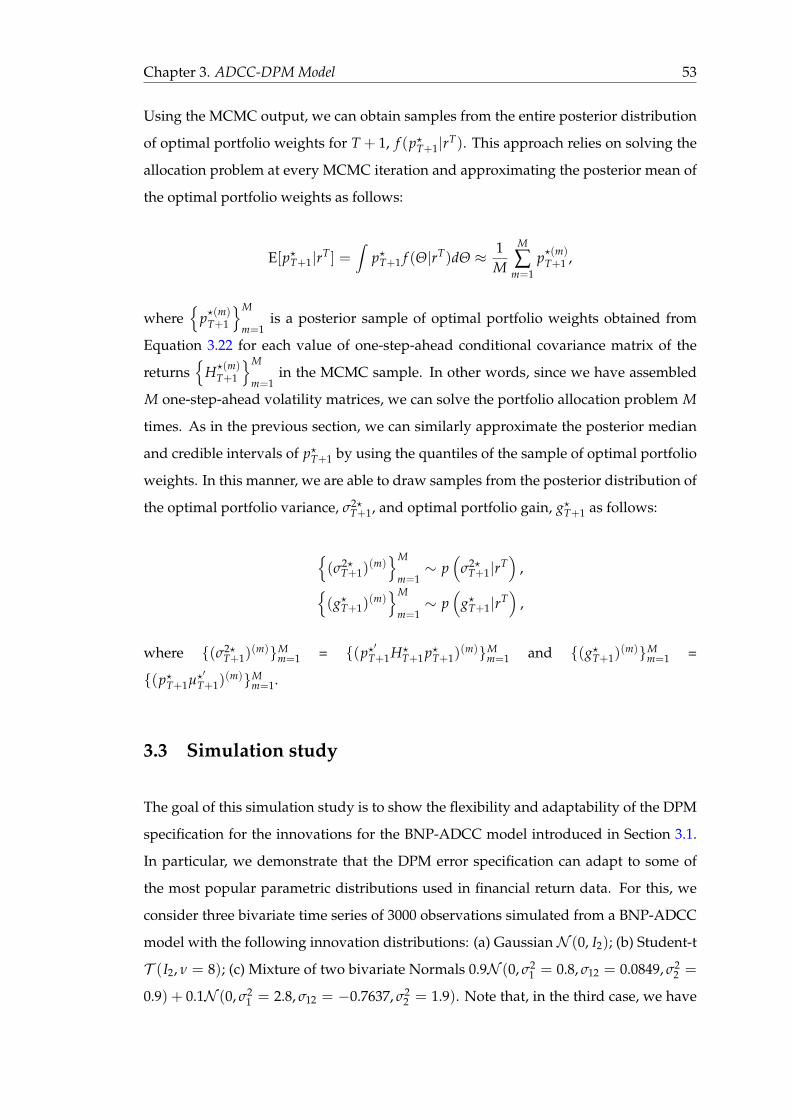
Chapter 3. ADCC-DPM Model 53
Using the MCMC output, we can obtain samples from the entire posterior distribution
of optimal portfolio weights for T + 1, f (p?T+1|rT). This approach relies on solving the
allocation problem at every MCMC iteration and approximating the posterior mean of
the optimal portfolio weights as follows:
E[p?T+1|rT] =∫
p?T+1 f (Θ|rT)dΘ ≈ 1M
M
∑m=1
p?(m)T+1 ,
where
p?(m)T+1
M
m=1is a posterior sample of optimal portfolio weights obtained from
Equation 3.22 for each value of one-step-ahead conditional covariance matrix of the
returns
H?(m)T+1
M
m=1in the MCMC sample. In other words, since we have assembled
M one-step-ahead volatility matrices, we can solve the portfolio allocation problem M
times. As in the previous section, we can similarly approximate the posterior median
and credible intervals of p?T+1 by using the quantiles of the sample of optimal portfolio
weights. In this manner, we are able to draw samples from the posterior distribution of
the optimal portfolio variance, σ2?T+1, and optimal portfolio gain, g?T+1 as follows:
(σ2?
T+1)(m)M
m=1∼ p
(σ2?
T+1|rT)
,(g?T+1)
(m)M
m=1∼ p
(g?T+1|rT
),
where (σ2?T+1)
(m)Mm=1 = (p?
′T+1H?
T+1 p?T+1)(m)M
m=1 and (g?T+1)(m)M
m=1 =
(p?T+1µ?′T+1)
(m)Mm=1.
3.3 Simulation study
The goal of this simulation study is to show the flexibility and adaptability of the DPM
specification for the innovations for the BNP-ADCC model introduced in Section 3.1.
In particular, we demonstrate that the DPM error specification can adapt to some of
the most popular parametric distributions used in financial return data. For this, we
consider three bivariate time series of 3000 observations simulated from a BNP-ADCC
model with the following innovation distributions: (a) GaussianN (0, I2); (b) Student-t
T (I2, ν = 8); (c) Mixture of two bivariate Normals 0.9N (0, σ21 = 0.8, σ12 = 0.0849, σ2
2 =
0.9) + 0.1N (0, σ21 = 2.8, σ12 = −0.7637, σ2
2 = 1.9). Note that, in the third case, we have
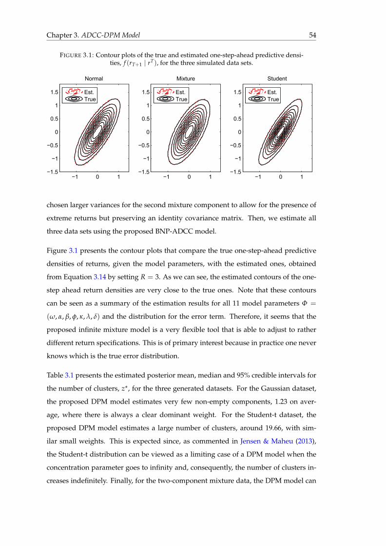
Chapter 3. ADCC-DPM Model 54
FIGURE 3.1: Contour plots of the true and estimated one-step-ahead predictive densi-ties, f (rT+1 | rT), for the three simulated data sets.
Normal
−1 0 1−1.5
−1
−0.5
0
0.5
1
1.5 Est.True
Mixture
−1 0 1−1.5
−1
−0.5
0
0.5
1
1.5 Est.True
Student
−1 0 1−1.5
−1
−0.5
0
0.5
1
1.5 Est.True
chosen larger variances for the second mixture component to allow for the presence of
extreme returns but preserving an identity covariance matrix. Then, we estimate all
three data sets using the proposed BNP-ADCC model.
Figure 3.1 presents the contour plots that compare the true one-step-ahead predictive
densities of returns, given the model parameters, with the estimated ones, obtained
from Equation 3.14 by setting R = 3. As we can see, the estimated contours of the one-
step ahead return densities are very close to the true ones. Note that these contours
can be seen as a summary of the estimation results for all 11 model parameters Φ =
(ω, α, β, φ, κ, λ, δ) and the distribution for the error term. Therefore, it seems that the
proposed infinite mixture model is a very flexible tool that is able to adjust to rather
different return specifications. This is of primary interest because in practice one never
knows which is the true error distribution.
Table 3.1 presents the estimated posterior mean, median and 95% credible intervals for
the number of clusters, z?, for the three generated datasets. For the Gaussian dataset,
the proposed DPM model estimates very few non-empty components, 1.23 on aver-
age, where there is always a clear dominant weight. For the Student-t dataset, the
proposed DPM model estimates a large number of clusters, around 19.66, with sim-
ilar small weights. This is expected since, as commented in Jensen & Maheu (2013),
the Student-t distribution can be viewed as a limiting case of a DPM model when the
concentration parameter goes to infinity and, consequently, the number of clusters in-
creases indefinitely. Finally, for the two-component mixture data, the DPM model can
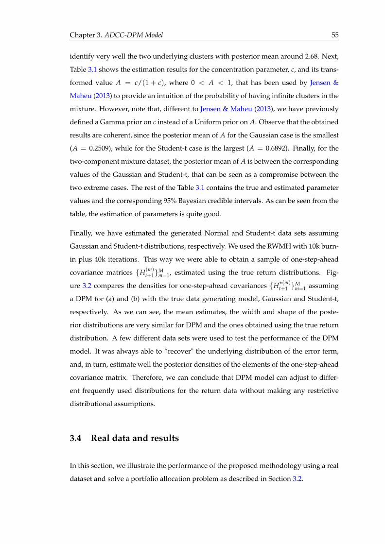
Chapter 3. ADCC-DPM Model 55
identify very well the two underlying clusters with posterior mean around 2.68. Next,
Table 3.1 shows the estimation results for the concentration parameter, c, and its trans-
formed value A = c/(1 + c), where 0 < A < 1, that has been used by Jensen &
Maheu (2013) to provide an intuition of the probability of having infinite clusters in the
mixture. However, note that, different to Jensen & Maheu (2013), we have previously
defined a Gamma prior on c instead of a Uniform prior on A. Observe that the obtained
results are coherent, since the posterior mean of A for the Gaussian case is the smallest
(A = 0.2509), while for the Student-t case is the largest (A = 0.6892). Finally, for the
two-component mixture dataset, the posterior mean of A is between the corresponding
values of the Gaussian and Student-t, that can be seen as a compromise between the
two extreme cases. The rest of the Table 3.1 contains the true and estimated parameter
values and the corresponding 95% Bayesian credible intervals. As can be seen from the
table, the estimation of parameters is quite good.
Finally, we have estimated the generated Normal and Student-t data sets assuming
Gaussian and Student-t distributions, respectively. We used the RWMH with 10k burn-
in plus 40k iterations. This way we were able to obtain a sample of one-step-ahead
covariance matrices H(m)t+1M
m=1, estimated using the true return distributions. Fig-
ure 3.2 compares the densities for one-step-ahead covariances H?(m)t+1 M
m=1 assuming
a DPM for (a) and (b) with the true data generating model, Gaussian and Student-t,
respectively. As we can see, the mean estimates, the width and shape of the poste-
rior distributions are very similar for DPM and the ones obtained using the true return
distribution. A few different data sets were used to test the performance of the DPM
model. It was always able to “recover" the underlying distribution of the error term,
and, in turn, estimate well the posterior densities of the elements of the one-step-ahead
covariance matrix. Therefore, we can conclude that DPM model can adjust to differ-
ent frequently used distributions for the return data without making any restrictive
distributional assumptions.
3.4 Real data and results
In this section, we illustrate the performance of the proposed methodology using a real
dataset and solve a portfolio allocation problem as described in Section 3.2.

Chapter 3. ADCC-DPM Model 56
TABLE 3.1: Posterior means, medians and 95% credible intervals for the number ofnon-empty clusters z?, concentration parameter c, quantity A = c/(1 + c), and model
parameters for the three simulated data sets.
Gaussian Student-t 2 comp. mixtureTrue Mean 95% CI Mean 95% CI Mean 95% CIvalue Median Median Median
z? 1.2330 (1.0000, 3.0000) 19.6612 (9.0000, 33.0000) 2.6765 (2.0000, 5.0000)1.0000 19.0000 2.0000
c 0.3578 (0.0934, 0.8072) 2.5037 (0.9327, 5.0059) 0.4863 (0.1512, 1.0408)0.3252 2.3308 0.4462
A 0.2509 (0.0855, 0.4467) 0.6892 (0.4826, 0.8335) 0.3122 (0.1314, 0.5100)0.2454 0.6998 0.3085
ω1 0.01 0.0075 (0.0045, 0.0104) 0.0110 (0.0072, 0.0154) 0.0201 (0.0104, 0.0315)0.0077 0.0110 0.0201
ω2 0.01 0.0138 (0.0071, 0.0204) 0.0109 (0.0065, 0.0182) 0.0130 (0.0071, 0.0218)0.0142 0.0103 0.0118
α1 0.1 0.0595 (0.0383, 0.0858) 0.0970 (0.0740, 0.1277) 0.1473 (0.0808, 0.2570)0.0582 0.0953 0.1353
α2 0.08 0.0699 (0.0402, 0.0930) 0.0710 (0.0500, 0.0998) 0.0962 (0.0512, 0.1408)0.0716 0.0693 0.0944
β1 0.85 0.8625 (0.8388, 0.8816) 0.8244 (0.7920, 0.8481) 0.8426 (0.8076, 0.8710)0.8629 0.8262 0.8441
β2 0.88 0.8695 (0.8478, 0.8946) 0.8727 (0.8539, 0.8888) 0.8939 (0.8589, 0.9130)0.8686 0.8734 0.8952
φ1 0.025 0.0299 (0.0085, 0.0544) 0.0395 (0.0049, 0.0749) 0.0463 (0.0034, 0.0800)0.0285 0.0392 0.0475
φ2 0.025 0.0385 (0.0137, 0.0705) 0.0229 (0.0031, 0.0554) 0.0438 (0.0147, 0.0729)0.0373 0.0204 0.0443
κ 0.05 0.0504 (0.0366, 0.0681) 0.0501 (0.0347, 0.0648) 0.0615 (0.0407, 0.0878)0.0495 0.0503 0.0588
λ 0.9 0.8908 (0.8670, 0.9136) 0.8946 (0.8786, 0.9075) 0.8898 (0.8674, 0.9167)0.8903 0.8957 0.8884
δ 0.025 0.0221 (0.0015, 0.0475) 0.0312 (0.0098, 0.0536) 0.0265 (0.0011, 0.0551)0.0216 0.0311 0.0264
3.4.1 Estimation
We consider the daily price data of Apple Inc. company (PAt ) and NASDAQ Industrial
index (PNt ) from January 1, 2000 till May 7, 2012, obtained from Yahoo Finance. Then,
daily prices are transformed into daily logarithmic returns (in %), resulting in T = 3098
observations. Table 3.2 provides the basic descriptive statistics and Figure 3.3 illustrates
the dynamics of the log-returns.
As expected, Apple Inc. has higher overall variance because of the higher mean return.
Both returns do not exhibit any evidence of autoregressive behavior. Apple Inc. returns
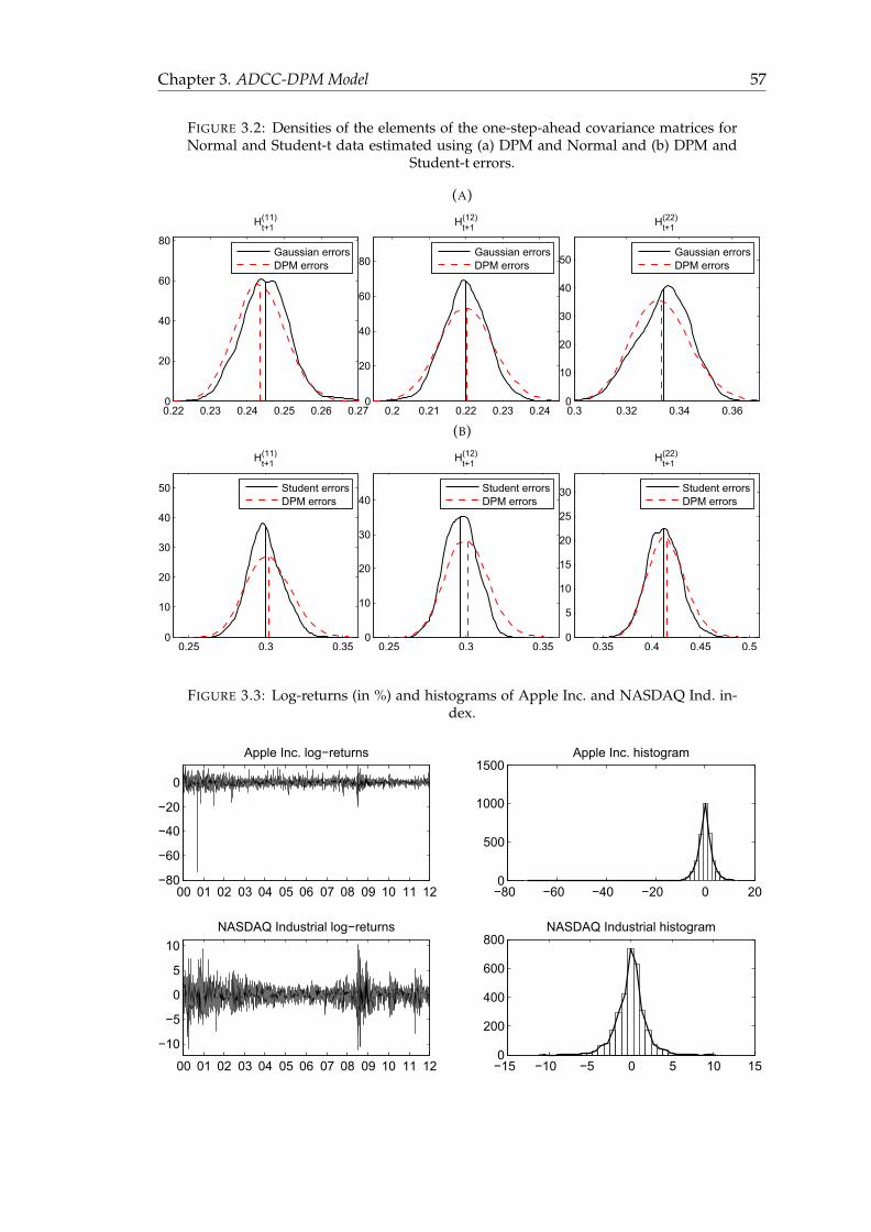
Chapter 3. ADCC-DPM Model 57
FIGURE 3.2: Densities of the elements of the one-step-ahead covariance matrices forNormal and Student-t data estimated using (a) DPM and Normal and (b) DPM and
Student-t errors.
(A)
0.22 0.23 0.24 0.25 0.26 0.270
20
40
60
80
Ht+1(11)
Gaussian errorsDPM errors
0.2 0.21 0.22 0.23 0.240
20
40
60
80
Ht+1(12)
Gaussian errorsDPM errors
0.3 0.32 0.34 0.360
10
20
30
40
50
Ht+1(22)
Gaussian errorsDPM errors
(B)
0.25 0.3 0.350
10
20
30
40
50
Ht+1(11)
Student errorsDPM errors
0.25 0.3 0.350
10
20
30
40
Ht+1(12)
Student errorsDPM errors
0.35 0.4 0.45 0.50
5
10
15
20
25
30
Ht+1(22)
Student errorsDPM errors
FIGURE 3.3: Log-returns (in %) and histograms of Apple Inc. and NASDAQ Ind. in-dex.
00 01 02 03 04 05 06 07 08 09 10 11 12−80
−60
−40
−20
0
Apple Inc. log−returns
−80 −60 −40 −20 0 200
500
1000
1500Apple Inc. histogram
00 01 02 03 04 05 06 07 08 09 10 11 12
−10
−5
0
5
10NASDAQ Industrial log−returns
−15 −10 −5 0 5 10 150
200
400
600
800NASDAQ Industrial histogram
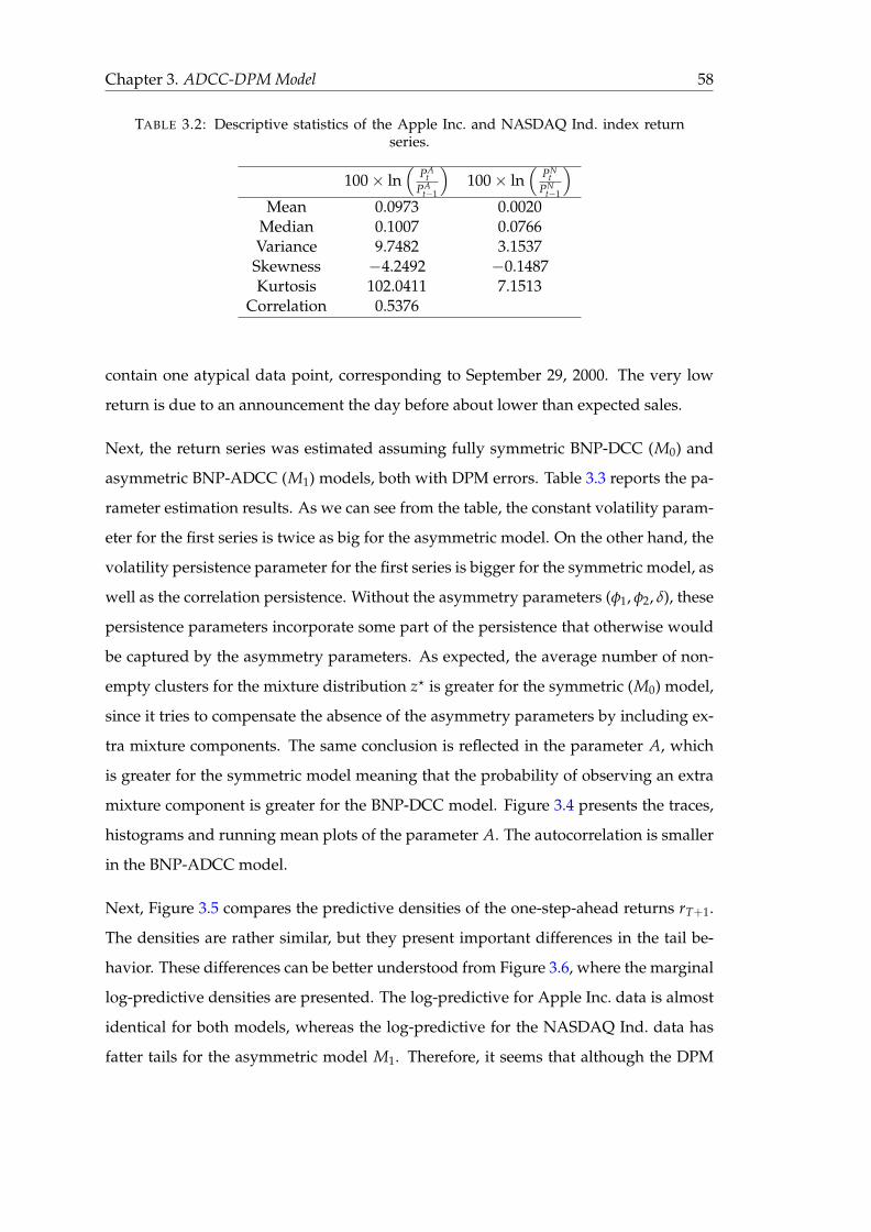
Chapter 3. ADCC-DPM Model 58
TABLE 3.2: Descriptive statistics of the Apple Inc. and NASDAQ Ind. index returnseries.
100× ln(
PAt
PAt−1
)100× ln
(PN
tPN
t−1
)Mean 0.0973 0.0020
Median 0.1007 0.0766Variance 9.7482 3.1537Skewness −4.2492 −0.1487Kurtosis 102.0411 7.1513
Correlation 0.5376
contain one atypical data point, corresponding to September 29, 2000. The very low
return is due to an announcement the day before about lower than expected sales.
Next, the return series was estimated assuming fully symmetric BNP-DCC (M0) and
asymmetric BNP-ADCC (M1) models, both with DPM errors. Table 3.3 reports the pa-
rameter estimation results. As we can see from the table, the constant volatility param-
eter for the first series is twice as big for the asymmetric model. On the other hand, the
volatility persistence parameter for the first series is bigger for the symmetric model, as
well as the correlation persistence. Without the asymmetry parameters (φ1, φ2, δ), these
persistence parameters incorporate some part of the persistence that otherwise would
be captured by the asymmetry parameters. As expected, the average number of non-
empty clusters for the mixture distribution z? is greater for the symmetric (M0) model,
since it tries to compensate the absence of the asymmetry parameters by including ex-
tra mixture components. The same conclusion is reflected in the parameter A, which
is greater for the symmetric model meaning that the probability of observing an extra
mixture component is greater for the BNP-DCC model. Figure 3.4 presents the traces,
histograms and running mean plots of the parameter A. The autocorrelation is smaller
in the BNP-ADCC model.
Next, Figure 3.5 compares the predictive densities of the one-step-ahead returns rT+1.
The densities are rather similar, but they present important differences in the tail be-
havior. These differences can be better understood from Figure 3.6, where the marginal
log-predictive densities are presented. The log-predictive for Apple Inc. data is almost
identical for both models, whereas the log-predictive for the NASDAQ Ind. data has
fatter tails for the asymmetric model M1. Therefore, it seems that although the DPM
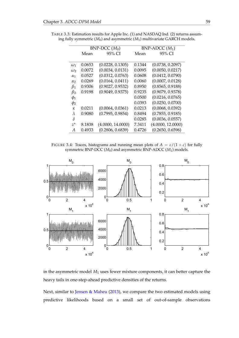
Chapter 3. ADCC-DPM Model 59
TABLE 3.3: Estimation results for Apple Inc. (1) and NASDAQ Ind. (2) returns assum-ing fully symmetric (M0) and asymmetric (M1) multivariate GARCH models.
BNP-DCC (M0) BNP-ADCC (M1)Mean 95% CI Mean 95% CI
ω1 0.0653 (0.0228, 0.1305) 0.1344 (0.0738, 0.2097)ω2 0.0072 (0.0034, 0.0131) 0.0095 (0.0050, 0.0217)α1 0.0527 (0.0312, 0.0763) 0.0608 (0.0412, 0.0790)α2 0.0269 (0.0164, 0.0411) 0.0060 (0.0007, 0.0128)β1 0.9306 (0.9027, 0.9532) 0.8950 (0.8565, 0.9188)β2 0.9198 (0.9049, 0.9375) 0.9235 (0.9079, 0.9378)φ1 0.0500 (0.0216, 0.0765)φ2 0.0393 (0.0250, 0.0700)κ 0.0211 (0.0064, 0.0361) 0.0213 (0.0068, 0.0392)λ 0.9080 (0.7995, 0.9854) 0.8494 (0.7855, 0.9185)δ 0.0285 (0.0036, 0.0557)z? 8.1838 (4.0000, 14.0000) 7.3411 (4.0000, 12.0000)A 0.4933 (0.2806, 0.6839) 0.4726 (0.2650, 0.6596)
FIGURE 3.4: Traces, histograms and running mean plots of A = c/(1 + c) for fullysymmetric BNP-DCC (M0) and asymmetric BNP-ADCC (M1) models.
0 2 4x 10⁴
0
0.5
1M0
0 0.5 10
2000
4000
6000
M0
0 2 4x 10⁴
0.2
0.4
0.6
0.8M0
0 2 4x 10⁴
0
0.5
1M1
0 0.5 10
2000
4000
6000
M1
0 2 4x 10⁴
0.2
0.4
0.6
0.8M1
in the asymmetric model M1 uses fewer mixture components, it can better capture the
heavy tails in one-step-ahead predictive densities of the returns.
Next, similar to Jensen & Maheu (2013), we compare the two estimated models using
predictive likelihoods based on a small set of out-of-sample observations
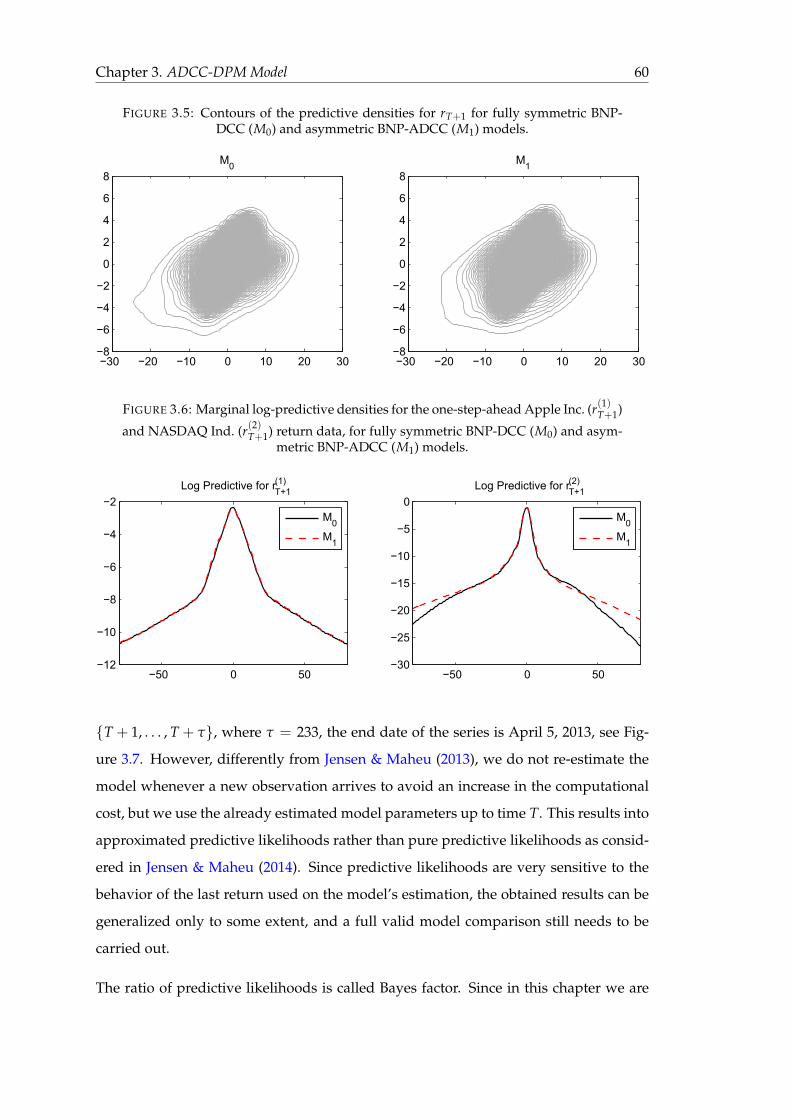
Chapter 3. ADCC-DPM Model 60
FIGURE 3.5: Contours of the predictive densities for rT+1 for fully symmetric BNP-DCC (M0) and asymmetric BNP-ADCC (M1) models.
M0
−30 −20 −10 0 10 20 30−8
−6
−4
−2
0
2
4
6
8M1
−30 −20 −10 0 10 20 30−8
−6
−4
−2
0
2
4
6
8
FIGURE 3.6: Marginal log-predictive densities for the one-step-ahead Apple Inc. (r(1)T+1)
and NASDAQ Ind. (r(2)T+1) return data, for fully symmetric BNP-DCC (M0) and asym-metric BNP-ADCC (M1) models.
−50 0 50−12
−10
−8
−6
−4
−2Log Predictive for rT+1
(1)
M0M1
−50 0 50−30
−25
−20
−15
−10
−5
0Log Predictive for rT+1
(2)
M0M1
T + 1, . . . , T + τ, where τ = 233, the end date of the series is April 5, 2013, see Fig-
ure 3.7. However, differently from Jensen & Maheu (2013), we do not re-estimate the
model whenever a new observation arrives to avoid an increase in the computational
cost, but we use the already estimated model parameters up to time T. This results into
approximated predictive likelihoods rather than pure predictive likelihoods as consid-
ered in Jensen & Maheu (2014). Since predictive likelihoods are very sensitive to the
behavior of the last return used on the model’s estimation, the obtained results can be
generalized only to some extent, and a full valid model comparison still needs to be
carried out.
The ratio of predictive likelihoods is called Bayes factor. Since in this chapter we are

Chapter 3. ADCC-DPM Model 61
FIGURE 3.7: Log-returns (in %) of Apple Inc. and NASDAQ Ind. index for t =3099, . . . , 3331.
12/05 12/06 12/08 12/09 12/11 12/12 13/02 13/04
−10
−5
0
5
Apple Inc. log−returns
12/05 12/06 12/08 12/09 12/11 12/12 13/02 13/04
−10
−5
0
5
NASDAQ Industrial log−returns
considering approximated predictive likelihoods, we will refer as pseudo Bayes factor
to the resulting ratios. As seen in Kass & Raftery (1995), the predictive likelihood for
the ith data point, given the kth model, can be obtained as
p(rT+i|rT+i−1, Mk) =∫
p(rT+i|rT+i−1, Mk, Θk)π(Θk|rT+i−1, Mk)dΘk,
where Θk is a set of parameters associated with the kth model. Since this integral is not
analytically tractable, we can approximate it using the MCMC output:
p(rT+i|rT+i−1, Mk) =1M
M
∑m=1
p(rT+i|rT+i−1, Mk, Θ(m)k ), for i = 1, 2, . . . , τ,
and then calculate the sum of the logarithms over the entire out-of-sample period:
log p(rT+1, . . . , rT+τ|Mk) =τ
∑i=1
log p(rT+i|rT+i−1, Mk).
Table 3.4 presents the cumulative approximated log-predictive likelihood for the two
models using τ = 233 out-of-sample observations. The log of the pseudo Bayes factor
can be obtained as a difference of the likelihoods:
log BF10 = log p(rT+1, . . . , rT+τ|M1)− log p(rT+1, . . . , rT+τ|M0),
where BFij represents a pseudo Bayes Factor comparing models i and j. As seen in
Kass & Raftery (1995), if 2 log BF10 ≥ 10, then M1 is strongly preferred to M0, since the

Chapter 3. ADCC-DPM Model 62
FIGURE 3.8: Posterior distributions of one-step-ahead volatilities for fully symmetricBNP-DCC (M0) and asymmetric BNP-ADCC (M1) models.
4 5 6 7 80
0.2
0.4
0.6
0.8
Ht+1*(1,1)
M0M1
0.5 1 1.5 2 2.50
1
2
3
4
Ht+1*(1,2)
M0M1
0.5 1 1.5 20
1
2
3
4
5
Ht+1*(2,2)
M0M1
former can predict the data better. In our case, 2 log BF10 = 9.9876, which favors the
fully asymmetric BNP-ADCC model.
TABLE 3.4: Cumulative log-predictive likelihoods for fully symmetric BNP-DCC (M0)and asymmetric BNP-ADCC (M1) models.
Model log p(rT+1, . . . , rT+τ|rT)
M0 -751.5094
M1 -746.5156
# of out-of-sample obs. τ = 233
Figure 3.8 draws the posterior densities of the volatilities and Table 3.5 presents the pos-
terior means, medians and confidence intervals for the elements of the one-step-ahead
volatility matrix. These are obtained using Equation 3.17 and the explanations given
in Section 3.1.3. Even though the posterior densities are of similar shape, the CI width
in all cases is smaller for the asymmetric model M1. It seems that by incorporating the
asymmetric assumption in the model we may obtain more precision in the predicted
volatilities and, consequently, in optimal portfolio weights and variances.
Finally, we have performed a sensitivity analysis on the posterior distribution of A =
c/(1 + c) and number of non-empty clusters z? by changing the hyper-parameters of
the concentration parameter c. In the simulation study and real data application we
have assumed c ∼ G(4, 4). In the sensitivity analysis we have tried two more combina-
tions: c ∼ G(1.5, 1) and c ∼ G(1/6, 1/3), such that a priori c would center at 0.5 and 1.5,
respectively. Table 3.6, Figure 3.9 and Figure 3.10 present the estimation results, which

Chapter 3. ADCC-DPM Model 63
TABLE 3.5: Posterior means, medians and confidence intervals for the elements of theone-step-ahead volatility matrix for fully symmetric BNP-DCC (M0) and asymmetric
BNP-ADCC (M1) models.
BNP-DCC (M0) BNP-ADCC (M1)Mean 95% HPD Mean 95% HPD
Median MedianH?(1,1)
T+1 6.0656 (4.8345, 7.1482) 6.4182 (5.3852, 7.4298)6.0780 6.4377
H?(1,2)T+1 1.4350 (1.0478, 1.7431) 1.6296 (1.3340, 1.8923)
1.4614 1.6504H?(2,2)
T+1 1.2346 (0.9647, 1.4132) 1.4369 (1.2345, 1.6322)1.2636 1.4469
FIGURE 3.9: Posterior distributions for A = c/(1 + c) and a number of non-emptyclusters z? for different hyper-parameters for c ∼ G(a0, b0) for BNP-ADCC model for
Apple-NASDAQ data.
0 0.2 0.4 0.6 0.8 1 1.20
1
2
3
4Posterior of A
G(4,4)G(1.5,1)G(1/6,1/3)
0 5 10 15 200
0.05
0.1
0.15
0.2Posterior of z*
G(4,4)G(1.5,1)G(1/6,1/3)
seem to be rather robust to the changes in hyper-parameters for the prior of c as long
as the priors are not very informative.
TABLE 3.6: Posterior means and 95% credible intervals for A = c/(1 + c) and a num-ber of non-empty clusters z? for different hyper-parameters for c ∼ G(a0, b0) for BNP-
ADCC model for Apple-NASDAQ data.
c ∼ G(4, 4) c ∼ G(1.5, 1) c ∼ G(1/6, 1/3)Mean of A 0.4726 0.4766 0.4588
95% CI of A (0.2650, 0.6596) (0.2011, 0.7305) (0.1648, 0.7296)Mean of z? 7.3411 7.4071 7.6391
95% CI of z? (4, 12) (4, 14) (4, 14)

Chapter 3. ADCC-DPM Model 64
FIGURE 3.10: Prior and posterior distributions for c for BNP-ADCC model for Apple-NASDAQ data.
0 1 2 3 4 50
0.5
1
G(4,4)G(1.5,1)G(1/6,1/3)
0 1 2 3 4 50
0.5
1
Posterior of cPrior c~G(4,4)
0 1 2 3 4 50
0.5
1
Posterior of cPrior c~G(1.5,1)
0 1 2 3 4 50
0.5
1
Posterior of cPrior c~G(1/6,1/3)
3.4.2 Portfolio allocation
Here we are interested in estimating the GMV optimal portfolio of the two real assets,
without the short-sale constraint, using the procedure described in Section 3.2. Firstly,
we will make predictions on the optimal one-step-ahead portfolio and then, we will
consider all the 233 out-of-sample future observations, adjusting the optimal portfolio
weights at each time period. Throughout the portfolio allocation exercise, we report
only the first portfolio weight p?(1)T+1, as the other can be obtained as p?(2)T+1 = 1− p?(1)T+1.
The estimation results for the T + 1 period are presented in Table 3.7 and the poste-
rior densities for optimal portfolio weights and variances can be seen in Figure 3.11.
The point estimates for the optimal portfolio weights for T + 1 period are very similar,
however, the asymmetric model estimates greater portfolio variance for T + 1 since the
estimated one-step-ahead volatilites for the BNP-ADCC model are greater. However,
note that, as before, the CI width is smaller for the M1 model.
TABLE 3.7: Posterior mean, median and 95% credible intervals for the optimal one-step-ahead portfolio weight and variance.
BNP-DCC (M0) BNP-ADCC (M1)Mean 95% CI Mean 95% CI
Median Medianp?T+1 -0.0457 (-0.0907, -0.0011) -0.0428 (-0.0869, 0.0017)
-0.0457 -0.0426σ2?
T+1 1.2234 (1.1570, 1.5924) 1.4266 (1.5175, 1.7722)1.2522 1.4352
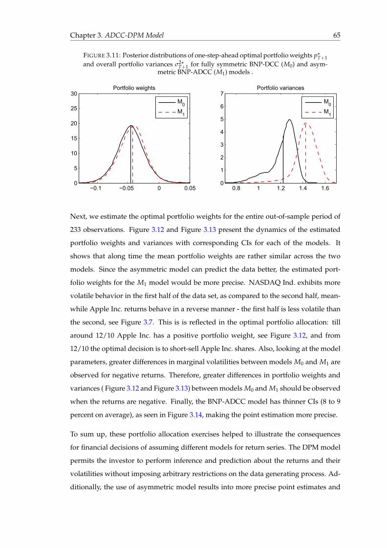
Chapter 3. ADCC-DPM Model 65
FIGURE 3.11: Posterior distributions of one-step-ahead optimal portfolio weights p?T+1and overall portfolio variances σ2?
T+1 for fully symmetric BNP-DCC (M0) and asym-metric BNP-ADCC (M1) models .
−0.1 −0.05 0 0.050
5
10
15
20
25
30Portfolio weights
M0M1
0.8 1 1.2 1.4 1.60
1
2
3
4
5
6
7Portfolio variances
M0M1
Next, we estimate the optimal portfolio weights for the entire out-of-sample period of
233 observations. Figure 3.12 and Figure 3.13 present the dynamics of the estimated
portfolio weights and variances with corresponding CIs for each of the models. It
shows that along time the mean portfolio weights are rather similar across the two
models. Since the asymmetric model can predict the data better, the estimated port-
folio weights for the M1 model would be more precise. NASDAQ Ind. exhibits more
volatile behavior in the first half of the data set, as compared to the second half, mean-
while Apple Inc. returns behave in a reverse manner - the first half is less volatile than
the second, see Figure 3.7. This is is reflected in the optimal portfolio allocation: till
around 12/10 Apple Inc. has a positive portfolio weight, see Figure 3.12, and from
12/10 the optimal decision is to short-sell Apple Inc. shares. Also, looking at the model
parameters, greater differences in marginal volatilities between models M0 and M1 are
observed for negative returns. Therefore, greater differences in portfolio weights and
variances ( Figure 3.12 and Figure 3.13) between models M0 and M1 should be observed
when the returns are negative. Finally, the BNP-ADCC model has thinner CIs (8 to 9
percent on average), as seen in Figure 3.14, making the point estimation more precise.
To sum up, these portfolio allocation exercises helped to illustrate the consequences
for financial decisions of assuming different models for return series. The DPM model
permits the investor to perform inference and prediction about the returns and their
volatilities without imposing arbitrary restrictions on the data generating process. Ad-
ditionally, the use of asymmetric model results into more precise point estimates and

Chapter 3. ADCC-DPM Model 66
FIGURE 3.12: A sequence of portfolio weights and their corresponding 95% CIs forτ = 1, . . . , 233 for fully symmetric BNP-DCC (M0) and asymmetric BNP-ADCC (M1)
models.
12/05 12/06 12/07 12/08 12/09 12/10 12/11 12/12 13/01 13/02 13/04−0.2
00.20.4
Portfolio weights
M
0
M1
12/05 12/06 12/07 12/08 12/09 12/10 12/11 12/12 13/01 13/02 13/04−0.2
00.20.4
Portfolio weights with 95% CIs for M0
12/05 12/06 12/07 12/08 12/09 12/10 12/11 12/12 13/01 13/02 13/04−0.2
00.20.4
Portfolio weights with 95% CIs for M1
FIGURE 3.13: A sequence of portfolio variances and their corresponding 95% CIs forτ = 1, . . . , 233 for fully symmetric BNP-DCC (M0) and asymmetric BNP-ADCC (M1)
models.
12/05 12/06 12/07 12/08 12/09 12/10 12/11 12/12 13/01 13/02 13/04012
Portfolio variances
M
0
M1
12/05 12/06 12/07 12/08 12/09 12/10 12/11 12/12 13/01 13/02 13/04012
Portfolio variance with 95% CIs for M0
12/05 12/06 12/07 12/08 12/09 12/10 12/11 12/12 13/01 13/02 13/04012
Portfolio variance with 95% CIs for M1

Chapter 3. ADCC-DPM Model 67
FIGURE 3.14: Mean cumsum of the of 95% CI width for the optimal portfolio weightsand variances for τ = 1, . . . , 233 for fully symmetric BNP-DCC (M0) and asymmetric
BNP-ADCC (M1) models.
12/05 12/07 12/08 12/10 12/12 13/02
0.09
0.1
0.11
0.12
0.13
Portfolio weights
M
0
M1
12/05 12/07 12/08 12/10 12/12 13/020.3
0.4
0.5
0.6
0.7
Portfolio variances
M0M1
better predictive performance. In the portfolio allocation context, adjusting portfolio
weights at each period might lead to high transaction costs, thus the investor will ad-
just her portfolio only if the expected utility after the adjustment minus the transaction
costs is greater than the expected utility without the adjustment.
On the other hand, an essential issue in choosing more complicated models versus the
simple ones is the ability to handle numerous assets, especially in financial applica-
tions, such as portfolio optimization. The DPM model is very flexible in this sense,
since the general specification described before contains numerous simplified models.
For example, it clearly contains the single Gaussian as a special case when the first mix-
ture weight is equal to one. Also, it is possible to impose a symmetric distribution for
the innovations by simply assuming that the mixture means are all equal and, in par-
ticular, it could be reasonable to impose µj = 0, for j = 1, 2, . . .. If we further assume
that the precision matrices are all diagonal, Λj = diag(λj1, . . . , λjK
), this will lead to
uncorrelated innovations. Finally, we could in addition assume that the diagonal ele-
ments of each precision matrix are all equal by considering Λj = λj IK. In this chapter
we have used the full version of the DPM model to illustrate the flexibility of it. The
adaptation of the model to these particular cases in order to simplify the problem of
many assets is straightforward from the theoretical point of view, but it might present
a heavy computational burden and some additional issues, such as convergence to a
stable posterior.
Chapter 3. ADCC-DPM Model 68
3.5 Conclusions
In this chapter we have proposed a Bayesian non-parametric approach for modeling
the distribution of multiple returns. We have used a BNP-ADCC model to explain the
individual volatilities and the time-varying correlations, taking into consideration the
asymmetries in individual assets’ volatilities, as well as in the correlations. The errors
are modeled using a location-scale mixture of infinite Gaussian distributions that has
been shown to allow for a great flexibility in the return distribution in terms of skew-
ness and kurtosis. An MCMC method has been presented for model estimation and
prediction. For that, DPM prior has been given to the infinite mixture of multivariate
Gaussian distribution. We have presented a short simulation study that illustrates the
differences arising from different assumptions for the errors and shows the adaptability
of the DPM model. The simulation results suggest that the proposed approach appears
to be able to fit adequately several frequently used distributions. Finally, we have pre-
sented a real data application that compares the proposed BNP-ADCC with a fully
symmetric BNP-DCC model by using return series of Apple Inc. and NASDAQ Indus-
trial index. Model comparison via approximated log-predictive likelihood favors the
asymmetric BNP-ADCC, which also produces thinner credible intervals for one-step-
ahead volatilities. Additionally, we have employed the proposed approach to solve a
portfolio allocation problem. The explained methodology and obtained results are not
limited to this specific risk management problem and could be expanded into various
other topics in applied finance and risk management.

Chapter 4
A Bayesian Non-Parametric
Approach to a MSSV Model with
Particle Learning
The previously reviewed Stochastic Volatility model, as introduced by Taylor (1982),
allows for time-varying volatility but it is unable to capture the usual heavy-tailed be-
havior of conditional distribution of the returns, since they are assumed to be Gaussian.
One alternative is to abandon parametric assumptions for the returns altogether and
consider a semi-parametric SV model, where the distribution of the returns is modeled
non-parametrically, at the same time conserving the parametric discrete representation
of the SV model.
Bayesian non-parametric approach in SV models is quite a new field of research, with
growing popularity due to its flexibility and superior performance, see Jensen & Maheu
(2010, 2014) and Delatola & Griffin (2011, 2013). In these works it is assumed that the
distribution of the returns follows an infinite mixture of Normals via Dirichlet Process
Mixture (DPM) models (see Ferguson 1983 and Lo 1984, among others) and Bayesian
estimation is performed using MCMC methods. The MCMC approach for SV models is
the usual methodology since the seminal work by Jacquier et al. (1994), where Bayesian
inference for standard SV models was firstly developed. However, MCMC methods in
general are computationally demanding and inherently non-sequential (Lopes & Pol-
son 2010). Alternatively, one can rely on Sequential Monte Carlo (SMC) methods, also
69

Chapter 4. MSSV-DPM with PL 70
known as particle filters, that allow for on-line type inference by updating the posterior
distribution as the new data is observed.
Therefore, in this chapter we use SMC methods for Bayesian non-parametric SV models
which allows us to incorporate new information on-line, i.e. as it arrives. In particular,
we make use of the PL approach, which is a particle based method, firstly introduced
by Carvalho, Johannes, Lopes & Polson (2010). Differently from other particle methods,
it does not suffer from particle degeneracy. It also makes model comparison easy, since
at each step we have the predictive likelihood as a by-product. PL methods have been
shown to outperform the existing particle filtering alternatives and to be a competitor
to MCMC, see Lopes et al. (2011).
In the first part of the chapter we design a PL algorithm for a SV model with DPM
innovations, referred to as a SV-DPM, similar to that of Delatola & Griffin (2011), and
compare the performance of the algorithm to MCMC. We find that PL performs as well
as MCMC, but, as commented above, the PL method provides the advantage of easily
incorporating the information from the new observation, while MCMC requires to re-
run the algorithm again.
In the second part of the chapter we augment the SV-DPM model by incorporating
Markov switching jumps, as seen in So et al. (1998) and Carvalho & Lopes (2007), re-
sulting into a new MSSV-DPM model. We extend the previously developed PL algo-
rithm to this new model and apply it on simulated data. Then, the performance of the
new MSSV-DPM model is compared with the SV-DPM specification using real financial
time series and we obtain that the new model provides better predictive power in the
tails of the distribution.
The chapter is structured as follows. Section 4.1 presents the linearized SV model with
non-parametric errors and compares the estimation output for the SV-DPM model by
using PL and MCMC. Then, Section 4.2 introduces a new MSSV-DPM model and de-
signs a PL algorithm for inference and prediction. Section 4.3 compares the perfor-
mance of the two non-parametric models by using real data. Finally, Section 4.4 con-
cludes.

Chapter 4. MSSV-DPM with PL 71
4.1 SV-DPM Model
In this section we briefly review a commonly used version of the standard stochastic
volatility model with Normal errors. We then drop the normality hypothesis and intro-
duce a novel particle learning scheme to perform sequential Bayesian learning in the
class of SV model with Dirichlet Process Mixture models innovations (SV-DPM). We
show, via synthetic examples, that our particle filter performs similarly to the standard
MCMC scheme, with the advantage of producing online inference and, as a by product,
online model comparison/selection statistics.
Normal errors
The standard SV model looks as follows:
yt = exp ht/2 vt,
ht = α + βht−1 + τηt,
where we impose |β| < 1 for the stationarity of the volatilities; vt and ηt are the error
terms, such that ηt ∼ N (0, 1) and the distribution of the vt with zero mean and unit
variance takes many different forms in the existing literature: from a standard Normal,
to heavy-tailed Student-t and others (see Kim et al. 1998, Chib et al. 2002, for example).
Kim et al. (1998) proposed linearlization of the standard SV model by defining rt =
log y2t and εt = log v2
t , resulting into the following dynamic linear model:
rt = ht + εt, where εt ∼ F , (4.1)
ht = α + βht−1 + τηt, where ηt ∼ N (0, 1). (4.2)
Observe that the distribution of εt is a log χ21 if vt is Normally distributed. Kim et al.
(1998) and Omori et al. (2007) use carefully tuned finite mixtures of Normals to ap-
proximate the distribution of log χ21 and use a data augmentation argument to propose
fast MCMC schemes that jointly sample h1, . . . , hT based on the well-known forward
filtering, backward sampling (FFBS) algorithm of Carter & Kohn (1994) and Frühwirth-
Schnatter (1994).
Chapter 4. MSSV-DPM with PL 72
However, the recent literature is abundant in showing that the distribution of vt has
heavier tails than Normal, rendering the above approximations useless. Below we in-
troduce the simple linearlized SV model with non-parametric errors to model the un-
known return distribution.
Non-Normal errors
Delatola & Griffin (2011, 2013), for example, propose to approximate the log-square of
the unknown return distribution εt ∼ F as an infinite mixture of Normals by relying
on DPM models. The simple SV-DPM model presented in this section is of the same
spirit as the model in Delatola & Griffin (2011).
Another important issue concerns the moments of the distribution of εt. Even though
the original errors vt are generated by a process with zero mean and unit variance,
the resulting moments of εt can vary greatly, depending on the distribution of vt. For
example, if vt ∼ N (0, 1), then E[εt] = −1.272, V[εt] = 4.946, S[εt] = −1.539 and
K[εt] = 7.015, where E[·], V[·], S[·] and K[·] denote mean, variance, skewness and
kurtosis, respectively. On the other hand, if vt ∼ ST (7), scaled in such a way that
E[vt] = 0 and V[vt] = 1, then E[εt] = −1.428, V[εt] = 5.218, S[εt] = −1.404 and
K[εt] = 6.583. However, Student-t and Normal are not the only possible distributions
for the errors. There is an infinite number of possibilities for the distribution of the
error term, whose moments are impossible to “map" backwards in order to recover the
true error distribution. Actually, the main interest is usually not the distribution of the
error term, but filtering and predicting the volatilities of the returns, which are highly
sensitive to the choice of the error distribution.
The model specification in Equation 4.1 and Equation 4.2 is slightly different from the
one in Delatola & Griffin (2011), since we do not sum the constant volatility parameter
α into the mixture. We leave this constant separate since in Section 4.2 we augment the
model by considering two different volatility levels, i.e. αst , where st ∈ 0, 1.
Next, we do not specify a parametric model for the error density, but instead, we as-
sume a Dirichlet Process Mixture prior, firstly introduced by Lo (1984). DPM mod-
els have been widely used for modeling time-varying volatilities, see Jensen & Maheu

Chapter 4. MSSV-DPM with PL 73
(2010, 2013, 2014), Delatola & Griffin (2011, 2013), Kalli et al. (2013), and Ausín et al.
(2014). This type of approach is known as time-invariant (independent) DPM.
As seen in Escobar & West (1995), the DPM model has the following density function:
f (εt; G) =∫
k(εt; θt)dG(θt),
where k is some density kernel with parameters θt and the mixing distribution G has
a DP prior, denoted here by G ∼ DP(c, G0(θ; $)). Here the sub-index t in θt does not
mean time-varying parameters, but refers to the fact that at each time t the observation
εt comes from a different kernel density with some parameters θt, following the mixing
distribution G. Parameter c is called the concentration parameter and G0(θ; $) is called
the base distribution. The concentration parameter c can be interpreted as the prior
belief about the number of clusters in the mixture. Small values of c assume a priori an
infinite mixture model with a small number of components with large weights. On the
contrary, large values of c assume a priori an infinite mixture model with all the weights
being very small. c is also called a precision parameter and indicates how close G is to
the base distribution G0, where larger c indicates that G is closer to G0.
Gaussian kernel and conjugate base prior. Considering a Gaussian kernel density,
εt ∼ N (µt, σ2t ), the conjugate base prior G0(µ, σ2; $) is a Normal - Inverse Gamma
prior, denoted here by G0 ∼ NIG(µ, σ2; m0, V0, a0, a0σ20 ), such that µ|σ2 is Normal,
N (µ; m0, V0σ2) and σ2 is Inverse Gamma, IG(σ2; a0/2, a0σ20 /2). Here m0, V0, a0 and
a0σ20 are the hyper-parameters in $.
Define Φ =(α, β, τ2) as the set of parameters associated with the parametric part of
the model, Ω = (µ, σ2)(j)∞j=1 as a set of parameters associated with the distribution
of the error term, and Θ = (Φ, Ω) as a complete set of all model parameters. Therefore,
the model in Equation 4.1 and Equation 4.2 can be rewritten as follows:
rt|ht, Θ ∼ cc + t− 1
N (rt; µ0 + ht, σ20 ) +
1c + t− 1
L?t−1
∑j=1
nt−1,jN (rt; µj + ht, σ2j ), (4.3)
ht|ht−1, Θ ∼ N (ht; α + βht−1, τ2), (4.4)
Chapter 4. MSSV-DPM with PL 74
where nt,j is a number of observations assigned to jth component at time t and L?t is
a number of non-empty components in the mixture at time t. Given this missing in-
formation, the mixture becomes finite, where the maximum number of components
theoretically is limited by the number of observations. In practice, data tends to cluster,
meaning that some observations come from the same component, therefore L?t ≤ t.
4.1.1 MCMC for SV-DPM
The standard Bayesian estimation of SV models, parametric or non-parametric, relies
on MCMC methods, which, however, can be costly, because they have to consider a
sampler for latent volatilities.
Jensen & Maheu (2010) construct a MCMC scheme for their proposed SV-DPM model,
where latent volatilities are sampled via random length block sampler, which helps
to reduce correlation between draws. The authors found that the semi-parametric SV
model is more robust to non-Normal data and provides better forecasts. In another
paper, Jensen & Maheu (2014) consider an asymmetric SV-DPM model. The authors
extend their previous semi-parametric sampler to a bivariate setting, where the inno-
vations of the returns and volatilities are modeled jointly via infinite scale mixture of
bivariate Normals.
Meanwhile, Delatola & Griffin (2011) use a linearized version of SV model. Conditional
on knowing which mixture component the data belongs to, the linearized SV model is
just a Normal Dynamic Linear Model (NDLM) and the latent volatilities are updated
by FFBS (see the discussion at the end of Section 4.1). The remainder of the model pa-
rameters are sampled via an extension of Gibbs sampler, called hybrid Gibbs sampler.
In their subsequent paper, Delatola & Griffin (2013) consider an asymmetric SV model.
Same as before, they make use of the linearization and update the latent log-volatilities
via FFBS and the other parameters via Metropolis-Hastings. All above MCMC schemes
are costly in the context of SV models for at least two reasons: (1) the MCMC sampler
has to include a filter for latent volatilities, and (2) the sampler has to be re-run each
time a new observation arrives.
Chapter 4. MSSV-DPM with PL 75
4.1.2 PL for SV-DPM
In this section we present the algorithm to perform PL estimation for a SV model with
non-parametric errors. PL, which was firstly introduced by Carvalho, Johannes, Lopes
& Polson (2010), allows for sequential filtering, smoothing and parameter learning by
including state-sufficient statistics in a set of particles. For reviews of particle methods
in general, see Lopes & Tsay (2011) and Lopes & Carvalho (2013). For a more detailed
explanation of PL with illustrations refer to Carvalho, Johannes, Lopes & Polson (2010)
and Lopes et al. (2011), among others.
The priors for model parameters are chosen to be conditionally conjugate:
h0 ∼ N (c0, C0), σ2 ∼ IG(a0/2, a0σ20 /2), µ|σ2 ∼ N (m0, V0σ2), τ2 ∼ IG(b0/2, b0τ2
0 /2),
β|τ2 ∼ T N (−1,1)(mβ, Vβτ2), α ∼ N (mα, Vα). Here T N (a,b) represents Normal distri-
bution, truncated at a and b. c0, C0, a0, a0σ20 , m0, V0, b0, b0τ2
0 , mβ, Vβ, mα and Vα are
hyper-parameters. Then, a set of sufficient statistics St contains all updated hyper-
parameters, necessary for the parameter simulation, as well as filtered state variables,
which are of two kinds: the latent log-volatilities ht and the indicator variable kt, which
tells us to which mixture component the error data point belongs to. For t = 1 . . . , T
and for each particle (i) iterate through three steps:
1. Resampling.
Resample old particles (states, sufficient statistics and parameters) with weights
w ∝1
c + t− 1
L?t−1
∑j=0
nj fN(rt; α + βht−1 + µj, τ2 + σ2j ),
proportional to the predictive density of the returns (n0 = c). The components
of Θ = (α, β, τ2, µ1, . . . , µL?t−1
, σ21 , . . . , σ2
L?t−1) have been simulated at the end of the
previous period.
2. Sampling.
(a) Sample new log-volatilities ht from
p(ht|ht−1, Θ, n, L?t−1, rt) =
L?t−1
∑j=0
nj
c + t− 1N (ht; mhj, Vhj),
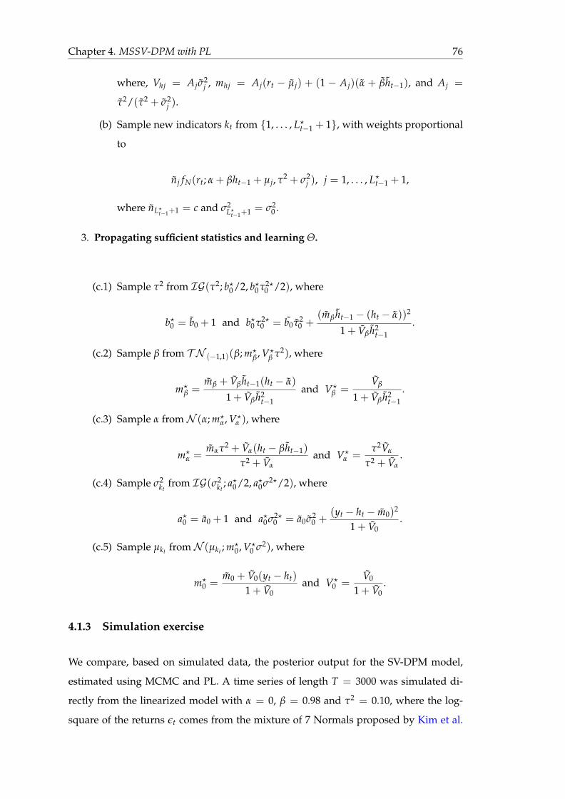
Chapter 4. MSSV-DPM with PL 76
where, Vhj = Ajσ2j , mhj = Aj(rt − µj) + (1 − Aj)(α + βht−1), and Aj =
τ2/(τ2 + σ2j ).
(b) Sample new indicators kt from 1, . . . , L?t−1 + 1, with weights proportional
to
nj fN(rt; α + βht−1 + µj, τ2 + σ2j ), j = 1, . . . , L?
t−1 + 1,
where nL?t−1+1 = c and σ2
L?t−1+1 = σ2
0 .
3. Propagating sufficient statistics and learning Θ.
(c.1) Sample τ2 from IG(τ2; b?0/2, b?0τ2?0 /2), where
b?0 = b0 + 1 and b?0τ2?0 = b0τ2
0 +(mβht−1 − (ht − α))2
1 + Vβh2t−1
.
(c.2) Sample β from T N (−1,1)(β; m?β, V?
β τ2), where
m?β =
mβ + Vβht−1(ht − α)
1 + Vβh2t−1
and V?β =
Vβ
1 + Vβh2t−1
.
(c.3) Sample α from N (α; m?α, V?
α ), where
m?α =
mατ2 + Vα(ht − βht−1)
τ2 + Vαand V?
α =τ2Vα
τ2 + Vα.
(c.4) Sample σ2kt
from IG(σ2kt
; a?0/2, a?0σ2?/2), where
a?0 = a0 + 1 and a?0σ2?0 = a0σ2
0 +(yt − ht − m0)2
1 + V0.
(c.5) Sample µkt from N (µkt ; m?0 , V?
0 σ2), where
m?0 =
m0 + V0(yt − ht)
1 + V0and V?
0 =V0
1 + V0.
4.1.3 Simulation exercise
We compare, based on simulated data, the posterior output for the SV-DPM model,
estimated using MCMC and PL. A time series of length T = 3000 was simulated di-
rectly from the linearized model with α = 0, β = 0.98 and τ2 = 0.10, where the log-
square of the returns εt comes from the mixture of 7 Normals proposed by Kim et al.
Chapter 4. MSSV-DPM with PL 77
(1998) to approximate the log χ21 distribution. Simulated returns can be recovered as
yt = exprt/2. MCMC results are obtained via Matlab code of Delatola & Griffin
(2011), which is available on Jim Griffin’s website1. The MCMC algorithm was run
for a total of 100k iterations, with the first 50k discarded as burn-in. The prior on the
persistence parameter is β ∼ T N (−1,1)(0.95, 0.1) and the prior for the volatility of the
volatility is τ2 ∼ IG(8, 0.24). The prior for the mixture components is different than
ours, since Delatola & Griffin (2011) use an alternative specification for the base distri-
bution (see Griffin 2010). Our PL algorithm, written in R, was run for a total of 300k
particles. The hyper-parameters in the PL scheme are set as c0 = 0, C0 = 0.1, mα = 0,
Vα = 0.01, mβ = 0.98, Vβ = 0.1, b0 = 6, b0τ20 = 1.20, a0 = 6, a0σ2
0 = 19, m0 = −1.27,
V0 = 5. The concentration parameter c in both codes is set to be equal to one. For vola-
tility process and the parameters we report the median particle as an estimate together
with 97.5% and 2.5% percentile particles for 95% credible intervals (CIs). For asym-
metric distributions instead of quantiles we are using the corresponding HPD (Highest
Posterior Density) intervals.
We have split the sample into three data sets of T = 1000, 2000 and 3000 observations.
In this way it is possible to see how PL is learning as compared to MCMC. The true
advantage of the PL procedure becomes evident at the moment when the new obser-
vation arrives. In MCMC setting we need to re-run the entire chain all over again in
order to incorporate this new information, meanwhile in PL we just add this new in-
formation to the existing output to obtain new updated parameters and states, which
is just a matter of seconds. The CPU time for both estimation approaches is presented
in Table 4.1.
TABLE 4.1: CPU time in seconds for MCMC and PL.
T MCMC (50k+50k) PL (300k particles)1000 233562000 517963000 80401 56999
Next, we compare the posterior output for both estimation methods graphically in Fig-
ure 4.1, Figure 4.2 and Figure 4.3 and Table 4.2. Figure 4.1 draws the estimated density
at T = 3000 for the log of the squared returns for PL and MCMC, compared to the true
1http://www.kent.ac.uk/smsas/personal/jeg28/index.htm
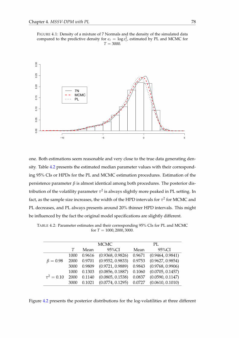
Chapter 4. MSSV-DPM with PL 78
FIGURE 4.1: Density of a mixture of 7 Normals and the density of the simulated datacompared to the predictive density for εt = log ε2
t , estimated by PL and MCMC forT = 3000.
−10 −5 0 5
0.00
0.05
0.10
0.15
0.20
0.25
0.30
7NMCMCPL
one. Both estimations seem reasonable and very close to the true data generating den-
sity. Table 4.2 presents the estimated median parameter values with their correspond-
ing 95% CIs or HPDs for the PL and MCMC estimation procedures. Estimation of the
persistence parameter β is almost identical among both procedures. The posterior dis-
tribution of the volatility parameter τ2 is always slightly more peaked in PL setting. In
fact, as the sample size increases, the width of the HPD intervals for τ2 for MCMC and
PL decreases, and PL always presents around 20% thinner HPD intervals. This might
be influenced by the fact the original model specifications are slightly different.
TABLE 4.2: Parameter estimates and their corresponding 95% CIs for PL and MCMCfor T = 1000, 2000, 3000.
MCMC PLT Mean 95%CI Mean 95%CI
1000 0.9616 (0.9368, 0.9826) 0.9671 (0.9464, 0.9841)β = 0.98 2000 0.9701 (0.9552, 0.9833) 0.9753 (0.9627, 0.9854)
3000 0.9809 (0.9721, 0.9889) 0.9843 (0.9768, 0.9906)1000 0.1303 (0.0856, 0.1887) 0.1060 (0.0705, 0.1457)
τ2 = 0.10 2000 0.1140 (0.0805, 0.1538) 0.0837 (0.0590, 0.1147)3000 0.1021 (0.0774, 0.1295) 0.0727 (0.0610, 0.1010)
Figure 4.2 presents the posterior distributions for the log-volatilities at three different

Chapter 4. MSSV-DPM with PL 79
FIGURE 4.2: Posterior distributions of the log-volatilities for MCMC and PL for T =1000, 2000 and 3000.
FIGURE 4.3: PL parameter estimates with 95% CI for one run of 300k particles, com-pared to the true parameter values.
α
β
τ

Chapter 4. MSSV-DPM with PL 80
data points T = 1000, 2000 and 3000. The posterior distributions for T = 2000 and
T = 3000 look identical among PL and MCMC. However, in order to obtain these
distributions MCMC had to be re-run three times for three "different“ data sets, mean-
while PL just incorporated new information sequentially and the posterior distribution
of any p(ht|rt) is readily available in the estimation output. Finally, Figure 4.3 draws
the PL parameter estimation path with 95% confidence bounds, as compared with the
true parameter values. As we can see, the parameter estimations become stable around
the 1500th observation. Also, there is no sign of particle degeneracy, which is a problem
in other particle filtering methods, see Rios & Lopes (2013) for example. Therefore, PL
can be seen as an efficient alternative to MCMC methods. Moreover, once the chain
has been run, at the arrival of the new observation the posterior distributions can be
updated at a very low computational cost.
In the next section we extend the non-parametric SV model to include Markov switch-
ing jumps and design a PL algorithm for inference and prediction.
4.2 MSSV-DPM Model
The simple SV model has some limitations such as it does not account for structural
changes in the volatility process, which we have to take into consideration, other-
wise the persistence parameter might be overestimated. For a brief review of Markov
switching GARCH and SV models refer to Section 2.1 and Section 2.2.
Consider a J-state Markov switching SV (MSSV) model, based on the model of So et al.
(1998), where the log-volatility equation is of the following form:
ht = αst + βht−1 + τηt, ηt ∼ N (0, 1),
where st are the regime variables following a two-state first order Markov Process:
pij = P [st = j|st−1 = i] , for i, j = 1, . . . , J.
As seen in Carvalho & Lopes (2007), we have to introduce the following reparametriza-
tion for αst in order to avoid identification issues:
Chapter 4. MSSV-DPM with PL 81
αst = γ1 +J
∑j=2
γj1 st ≥ j , γ1 ∈ < and γj > 0 for j > 1.
Here 1st ≥ j is an indicator function that takes values equal to one if st ≥ j and zero
otherwise (st < j).
In this section we consider a two-state MSSV model, as seen in Carvalho & Lopes
(2007), since it is a natural starting point. However, the a priori selection of number of
states might not fully capture the underlying data structure, since more regimes might
be necessary, especially after the 2007-2009 financial crisis. Therefore, a natural exten-
sion could be to compare models with different number of volatility states and select
the most appropriate one, as has been done by Bauwens et al. (2014) in MS-GARCH
setting, among many others. Therefore, in the case of only two regimes the st variables
follow a two-state first order Markov Process:
pij = P [st = j|st−1 = i] , for i, j = 0, 1.
And the αst reparametrization is as follows:
αst = γ0 + γ11 st = 1 , γ0 ∈ < and γ1 > 0,
where the indicator function 1st = 1 takes values equal to one if the volatility is in
the high state (st = 1) and zero otherwise (st = 0). We also need to define the transition
matrix between the states 0 and 1:
T =
P(st = 0|st−1 = 0) P(st = 1|st−1 = 0)
P(st = 0|st−1 = 1) P(st = 1|st−1 = 1)
=
p 1− p
1− q q
.
There are several papers that consider regime switching SV models in Bayesian con-
text. Kalimipalli & Susmel (2004) have proposed a two-factor SV model with regime
switching and estimated it using Gibbs sampler. They find that the high volatility per-
sistence is reduced when the regimes are incorporated in the model. Also, the authors
compare the new model with other two alternative two-factor models, simple SV and
GARCH, and find that SV always outperforms GARCH, both in sample and out of
Chapter 4. MSSV-DPM with PL 82
sample. The regime switching SV performs better than the simple SV in sample, how-
ever, out of sample, it is only marginally better. Lopes & Carvalho (2007) extend SV
model to multivariate case and present a Factor Stochastic Volatility (FSV) model with
Markov switching jumps. They construct a novel MCMC scheme for inference and find
that the new model can capture market crashes in an instantaneous way, as opposed
to the traditional FSV models. Carvalho & Lopes (2007) have constructed a sequential
Monte Carlo filter by combining auxiliary particle filter (APF) with the filter of Liu &
West (2001) to estimate a SV model with Markov switching regimes. They found that
in terms of prediction the Markov switching SV specification outperforms a simple SV
model.
Here we extend the SV-DPM model in Equation 4.3 and Equation 4.4 to accommodate
the above regime-shifting structure:
rt|ht, Θ ∼ cc + t− 1
N (rt; µ0 + ht, σ20 ) +
1c + t− 1
L?t−1
∑j=1
nt−1,jN (rt; µj + ht, σ2j ),
ht|ht−1, λt, Θ ∼ N (ht; γ0 + γ1λt + βht−1, τ2),
λt|Θ ∼ BER((1− p)1−λt−1 qλt−1
),
where BER(p) denotes a Bernoulli distribution with parameter p and λt is a Bernoulli
distributed state variable.
4.2.1 PL for MSSV-DPM
We extend the previous PL algorithm of SV-DPM for MSSV-DPM, by incorporating the
estimation of three extra parameters and filtering of one more state variable λt. The
set of the parameters for the parametric part of the model is Φ = (γ0, γ1, β, τ2, p, q).
Also, priors for the new parameters are: γ0 ∼ N (mγ0 , Vγ0), γ1 ∼ T N (0,+∞)(mγ1 , Vγ1),
p ∼ B(αp, βp) and q ∼ B(αq, βq). For t = 1 . . . , T and for each particle (i) iterate
through three steps:
1. Resampling.
Resample with weights proportional to the predictive density of the returns:

Chapter 4. MSSV-DPM with PL 83
w(i) ∝1
c + t− 1
L?t−1
∑j=1
nj fN(rt; γ0 + γ1λt−1 + βht−1 + µj, τ2 + σ2j )+
cc + t− 1
fN(rt; γ0 + γ1λt−1 + βht−1 + µ0, τ2 + σ20 ).
Here Θ = (γ0, γ1, β, τ2, p, q, µ1, . . . , µL?t−1
, σ21 , . . . , σ2
L?t−1) have been simulated at the
end of the previous period.
2. Sampling.
(a) Sample new states of the log-volatilities λt:
λt|λt−1, ht−1, Θ, rt ∼ BER(
z2
z1 + z2
),
where
z1 =1
c + t− 1
L?t−1
∑j=1
nj fN(rt; γ0 + βht−1 + µj, τ2 + σ2j )+
cc + t− 1
fN(rt; γ0 + βht−1 + µ0, τ2 + σ20 )× Pr(λt = 0|λt−1, Θ),
z2 =1
c + t− 1
L?t−1
∑j=1
nj fN(rt; γ0 + γ1λt−1 + βht−1 + µj, τ2 + σ2j )+
cc + t− 1
fN(rt; γ0 + γ1λt−1 + βht−1 + µ0, τ2 + σ20 )× Pr(λt = 1|λt−1, Θ).
Then call α = γ0 + γ1λt.
(b) Sample new log-volatilities ht:
p(ht|ht−1, Θ, n, L?t−1, rt) =
L?t−1
∑j=1
nj
c + t− 1N (ht; mhj, Vhj) +
cc + t− 1
N (ht; mh0, Vh0),
where
mhj =τ2(rt − µj) + σ2
j (α + βht−1)
τ2 + σ2j
and Vhj =σ2
j τ2
σ2j + τ2
.
For each particle we sample ht from a mixture of L?t−1 + 1 components with
the corresponding weights from the previous period.
(c) Sample new indicators kt from 1, . . . , L?t−1 + 1, with weights proportional
to:
Chapter 4. MSSV-DPM with PL 84
nj fN(rt; α + βht−1 + µj, τ2 + σ2j ), j = 1, . . . , L?
t−1,
where nL?t−1+1 = c and σ2
L?t−1+1 = σ2
0 .
3. Propagating sufficient statistics and learning Θ.
(c.1) Sample γ0 from N (γ0; m?γ0
, V?γ0), where
m?γ0
=mγ0 τ2 + Vγ0(ht − (γ1λt + βht−1))
τ2 + Vγ0
and V?γ0
=τ2Vγ0
τ2 + Vγ0
.
(c.2) Sample γ1 from T N (0,+∞)(γ1; m?γ1
, V?γ1), where
m?γ1
=mγ1 τ2 + Vγ1 λt(ht − (γ0 + βht−1))
Vγ1 λt + τ2and V?
γ1=
τ2Vγ1
τ2 + λtVγ1
.
Call α = γ0 + γ1λt.
(c.3) Sample p from B(p; α?p, β?
p), where
α?p = αp + 1 if λt = 0|λt−1 = 0 and β?
p = βp + 1 if λt = 1|λt−1 = 0.
(c.4) Sample q from B(q; α?q , β?
q), where
α?q = αq + 1 if λt = 1|λt−1 = 1 and β?
q = βq + 1 if λt = 0|λt−1 = 1.
(c.5) Sample τ2 from IG(τ2; b?0/2, b?0τ2?0 /2), where
b?0 = b0 + 1 and b?0τ2?0 = b0τ2
0 +(mβht−1 − (ht − α))2
1 + Vβh2t−1
.
(c.6) Sample β from T N (−1,1)(β; m?β, V?
β τ2), where
m?β =
mβ + Vβht−1(ht − α)
1 + Vβh2t−1
and V?β =
Vβ
1 + Vβh2t−1
.
(c.7) Sample σkt from IG(σ2kt
; a?0/2, a?0σ2?/2), where
a?0 = a0 + 1 and a?0σ2?0 = a0σ2
0 +(rt − ht − m0)2
1 + V0.
(c.8) Sample µkt from N (µkt ; m?0 , V?
0 σ2), where
m?0 =
m0 + V0(rt − ht)
1 + V0and V?
0 =V0
1 + V0.

Chapter 4. MSSV-DPM with PL 85
FIGURE 4.4: Simulated data: daily returns (top graph), true and estimated log-volatilities (middle graph) and true and estimated regimes (bottom graph).
0 500 1000 1500 2000 2500 3000
−4−2
02
4Daily Returns
Index
r
0 500 1000 1500 2000 2500 3000
−1.5
−0.5
0.5
Log Volatility (True in black & estimated in grey)
Time
0 500 1000 1500 2000 2500 3000
0.0
0.4
0.8
Volatility states (True in black & estimated in grey)
Time
4.2.2 Simulated data
In order to test the proposed model we use a simulated data set with the following
parameters: γ0 = −0.06, γ1 = 0.08, β = 0.92, τ2 = 0.01, p = 0.995, q = 0.995. The
errors follow a standard Normal distribution εt ∼ N (0, 1). The hyper-parameters are:
mγ0 = γ0, Vγ0 = γ20, mγ1 = γ1, Vγ1 = γ2
1, αp = 4, βp = 1, αq = 4, βq = 1, mβ = β,
Vβ = 0.1, b0 = 3, b0τ20 = 0.01, m0 = −1.2704, V0 = 5, a0 = 5 and a0σ2
0 = 15. We
estimate this data with MSSV-DPM model using PL, number of particles N = 300k.
The estimation results are presented in the Figure 4.4, Figure 4.5 and Figure 4.6.
Figure 4.4 top graph draws the simulated returns. The middle graph represents the true
realization of the log-volatility (in black) and the mean estimated filtered log-volatility
(in grey). The estimation of the latent log-volatility seems reasonable. The bottom
graph of the same figure draws the mean probability of being in a state one (st = 1).
As seen from the figure, PL takes some time to learn, since at first it is not able to
distinguish the regimes well. However, around observation 1000 the algorithm is able
to correctly identify the regimes with the overall miss-classification rate equal to 13%.

Chapter 4. MSSV-DPM with PL 86
FIGURE 4.5: Simulated data: true and estimated density for log-squared return distri-bution.
FIGURE 4.6: Simulated data: true and estimated parameters with 95% HPD intervals.
γ γ
− −
β τ

Chapter 4. MSSV-DPM with PL 87
FIGURE 4.7: Simulated data II: daily returns (top graph), true and estimated volatilities(middle graph) and true and estimated regimes (bottom graph).
−4−2
02
Daily log−returns (in %)0.
51.
52.
53.
5
Volatility (true in black & estimated in grey)
0.0
0.4
0.8
Volatility states (true in black & estimated in grey)
Figure 4.5 draws the true and estimated density for the log-squared returns, which is
log χ21. Finally, Figure 4.6 draws the sequential estimation of the model parameters and
their 95% HPD intervals. Overall, the obtained estimation results seem quite reasonable
and PL is able to correctly identify volatility regimes, filter log-volatilities, estimate
the density of the errors and the parameters in an efficient sequential manner. The
classification would become more troublesome once one of the regimes becomes less
persistent, and it would even worsen if both of the regimes become less persistent. This
would mean very frequent changes in volatility states that the model would not have
time to capture properly. See, for example, estimation results of another simulation
study in Figure 4.7, where the high volatility state regime is less persistent q = 0.950.
4.3 Real data application
In this section we present a real data application using return time series for various
financial assets, in particular one index - S&P500, one company - Ford - and one com-
modity - natural gas. The S&P500 prices are from Jan 2nd 1997 till Sept 9th 2014, Ford

Chapter 4. MSSV-DPM with PL 88
FIGURE 4.8: Daily log-returns (in %) and corresponding histograms for S&P500, Fordand Natural gas data.
−10
−50
510
Daily log−returns (in %) for S&P500 data
ene 1997 dic 2000 dic 2004 dic 2008 nov 2012
Histogram of S&P500 daily log−returns
−10 −5 0 5 10
040
080
0
−30
−10
10
Daily log−returns (in %) for Ford data
ene 1997 feb 2001 mar 2005 abr 2009 may 2013
Histogram of Ford daily log−returns
−30 −20 −10 0 10 20
020
060
0
−60
−20
2060
Daily log−returns (in %) for Natural gas data
ene 1997 jun 2001 ago 2005 oct 2009 nov 2013
Histogram of Natural gas daily log−returns
−60 −40 −20 0 20 40 60
040
080
0
from Jan 2nd 1997 till Sept 9th 2014 and Henry Hub natural gas spot prices (dollars per
million btu) from Jan 5th 1997 till Sept 9th 2014. The summary of descriptive statistics
can be seen in Table 4.3 and Figure 4.8.
TABLE 4.3: Descriptive statistics for S&P500, Ford and Gas data.
S&P500 Ford GasMean 0.0223 0.0182 0.0104
Median 0.0690 -0.0778 0.0668St.dev. 1.2752 2.8026 4.4554
Skewness -0.2237 -0.0220 0.7370Kurtosis 10.4789 15.8981 28.3024
T 4447 4329 4193
Next, we estimate the data with two non-parametric models, SV-DPM and MSSV-DPM.
The hyper-parameters for the priors are as follows: c0 = 0, C0 = 0.1, mα = 0, Vα =
Chapter 4. MSSV-DPM with PL 89
0.001, mβ = 0.95, Vβ = 0.1, b0 = 8, b0τ20 = 0.24, a0 = 6, a0σ2
0 = 18, m0 = −1.26, V0 = 5
for SV-DPM and mγ0 = −0.10, Vγ0 = 0.01, mγ1 = 0.20, Vγ1 = 0.04, αp = 7, βp = 1,
αq = 7, βq = 1, mβ = 0.95, Vβ = 0.01, b0 = 8, b0τ20 = 0.456, m0 = −1.26, V0 = 5, a0 = 6,
a0σ20 = 18 for MSSV-DPM. The codes were run for 500k particles each.
To compare the performance of the models, we use the average log-predictive score
(LPS) and average log-predictive tail score (LPTSα), which restrics attention to the
events in the upper 100α% of the empirical distribution of the squared returns, as seen
in Delatola & Griffin (2011). The LPS is defined as follows:
LPS = − 1T
T
∑t=1
log p(rt|rt−1),
and LPTSα is defined as:
LPTSα = − 1T∑
t=11rt > zα
T
∑t=1
1rt > zα log p(rt|rt−1),
where zα is the upper 100α percentile of the empirical distribution of rt. As Delatola &
Griffin (2011) point out, the LPTSα is not considered a proper scoring rule, however, it
can be very useful for understanding how the model performs in the tails.
The log-predictive densities are very easy to obtain in SMC setting, since they are a
by-product of the estimation procedure and, for each t = 1, . . . , T, are calculated as
log p(rt|rt−1) =1N
N
∑i=1
log p(rt|(Θ, ht, kt)(i)). (4.5)
Differently than in Delatola & Griffin (2011), there is no need to fix a certain Θ for
the calculation of the LPS and LPTSα, since we can account for parameter and state
uncertainty by using the approximation in Equation 4.5.
Next, we present the estimation results for the S&P500 data set. Figure 4.9 and Fig-
ure 4.10 present estimated predictive densities, filtered volatilities and volatility states
and Table 4.4 presents the estimated parameters. Figure 4.9 shows the estimated densi-
ties for the error term as compared to the frequently used mixture of 7 Normals, as an
approximation of log χ21. SV-DPM and MSSV-DPM models estimates are very similar to

Chapter 4. MSSV-DPM with PL 90
FIGURE 4.9: Estimated densities for the log-squared error term for SV-DPM andMSSV-DPM models.
−10 −5 0 5
0.00
0.05
0.10
0.15
0.20
0.25
0.30
7NSV−DPMMSSV−DPM
each other and different from the 7N approximation. This shows that the assumption of
Normality is very restrictive and in most cases incorrect. As we can see in Figure 4.10,
the filtered volatility for both models is very similar (second and third graphs). Ad-
ditionally, the MSSV-DPM model is able to identify some different volatility regimes,
especially in the second half of the data series when the algorithm had time to learn
(bottom graph). As for the parameter estimation in Table 4.4, the volatility persistence
parameter tends to be larger for the SV-DPM model, as expected, see So et al. (1998)
and Kalimipalli & Susmel (2004), among others.
TABLE 4.4: Parameter estimation for SV-DPM and MSSV-DPM models for S&P500data at time T.
SV-DPM MSSV-DPMMean 95%CI Mean 95%CI
α 0.0144 (0.0098, 0.0190) - -β 0.9792 (0.9747, 0.9837) 0.9474 (0.9383, 0.9550)τ2 0.0187 (0.0172, 0.0202) 0.0255 (0.0239, 0.0276)γ0 - - 0.0052 (-0.0010, 0.0131)γ1 - - 0.1279 (0.1069, 0.1497)p - - 0.9943 (0.9898, 0.9973)q - - 0.9585 (0.9352, 0.9782)

Chapter 4. MSSV-DPM with PL 91
FIGURE 4.10: Filtered volatilities and volatility states for S&P500 data for SV-DPMand MSSV-DPM models.
−10
010
Daily log−returns (in %)
ene 1997 may 1999 oct 2001 mar 2004 jul 2006 dic 2008 abr 2011 sep 2013
−11
3
Log−volatility (SV in black & MSSV in grey)
ene 1997 may 1999 oct 2001 mar 2004 jul 2006 dic 2008 abr 2011 sep 2013
020
40
Volatility (SV in black & MSSV in grey)
ene 1997 may 1999 oct 2001 mar 2004 jul 2006 dic 2008 abr 2011 sep 2013
0.0
0.6
MSSV volatility states
ene 1997 may 1999 oct 2001 mar 2004 jul 2006 dic 2008 abr 2011 sep 2013

Chapter 4. MSSV-DPM with PL 92
TABLE 4.5: LPS and LPTSα for SV-DPM and MSSV-DPM for S&P500 data.
SV-DPM MSSV-DPM differenceLPS 2.1907 2.2029 -0.0122
LPTS0.10 2.6444 2.6610 -0.0166LPTS0.05 2.9369 2.9282 0.0087LPTS0.01 3.6168 3.5068 0.1100
Table 4.5 presents the LPS and LPTSα for the S&P500 data. Same as in the paper by De-
latola & Griffin (2011), where the authors compare parametric and non-parametric SV
models, the LPS are very similar thus making the models virtually indistinguishable.
However, once we concentrate on the tails, the MSSV-DPM model tends to perform
better, especially if we consider the very extreme events (the 99th percentile).
Similar results can be seen in the estimation of the other two data sets, see Table 4.6,
Table 4.7, Table 4.8 and Table 4.9 and Figure 4.11 and Figure 4.12. For Ford and Natural
gas data the SV-DPM model estimates larger persistence parameter, same as in the
S&P500 data set. Also, the LPS for both models are very similar, but the differences
appear when we consider only the tails of the distribution.
TABLE 4.6: Parameter estimation for SV-DPM and MSSV-DPM models for Ford dataat time T.
SV-DPM MSSV-DPMMean 95%CI Mean 95%CI
α 0.0198 (-0.0238, 0.0264) - -β 0.9738 (0.9678, 0.9791) 0.9389 (0.9287, 0.9481)τ2 0.0274 (0.0171, 0.0366) 0.0474 (0.0442, 0.0509)γ0 - - 0.0013 (-0.0088, 0.0089)γ1 - - 0.0875 (0.0731, 0.1087)p - - 0.9944 (0.9909, 0.9974)q - - 0.9854 (0.9755, 0.9929)
To conclude, it seems that the SV-DPM and MSSV-DPM models tend to perform sim-
ilarly, if we consider the entire predictive distribution of the returns. However, the
identification of different volatility regimes becomes important if we consider the tails
of the distributions, where the MSSV-DPM model performs better. This is of major
interest not only in portfolio allocation setting, but also in risk measurement and man-
agement problems, where the agents are usually more interested in the tails than the
entire distribution.

Chapter 4. MSSV-DPM with PL 93
TABLE 4.7: LPS and LPTSα for SV-DPM and MSSV-DPM for Ford data.
SV-DPM MSSV-DPM differenceLPS 2.0718 2.0851 -0.0133
LPTS0.10 2.7639 2.7687 -0.0048LPTS0.05 3.1086 3.0956 0.0130LPTS0.01 4.1864 4.1007 0.0857
FIGURE 4.11: Filtered volatilities and volatility states for Ford data for SV-DPM andMSSV-DPM models.
−30
0
Daily log−returns (in %)
ene 1997 jun 1999 dic 2001 may 2004 oct 2006 abr 2009 sep 2011 feb 2014
−21
3
Log−volatility (SV in black & MSSV in grey)
ene 1997 jun 1999 dic 2001 may 2004 oct 2006 abr 2009 sep 2011 feb 2014
010
20
Volatility (SV in black & MSSV in grey)
ene 1997 jun 1999 dic 2001 may 2004 oct 2006 abr 2009 sep 2011 feb 2014
0.0
0.6
MSSV volatility states
ene 1997 jun 1999 dic 2001 may 2004 oct 2006 abr 2009 sep 2011 feb 2014

Chapter 4. MSSV-DPM with PL 94
FIGURE 4.12: Filtered volatilities and volatility states for Gas data for SV-DPM andMSSV-DPM models.
−60
060
Daily log−returns (in %)
ene 1997 sep 1999 abr 2002 oct 2004 may 2007 oct 2009 abr 2012
−30
2
Log−volatility (SV in black & MSSV in grey)
ene 1997 sep 1999 abr 2002 oct 2004 may 2007 oct 2009 abr 2012
010
20
Volatility (SV in black & MSSV in grey)
ene 1997 sep 1999 abr 2002 oct 2004 may 2007 oct 2009 abr 2012
0.2
0.6
MSSV volatility states
ene 1997 sep 1999 abr 2002 oct 2004 may 2007 oct 2009 abr 2012

Chapter 4. MSSV-DPM with PL 95
TABLE 4.8: Parameter estimation for SV-DPM and MSSV-DPM models for Gas data attime T.
SV-DPM MSSV-DPMMean 95%CI Mean 95%CI
α -0.0430 (-0.0481, -0.0342) - -β 0.9823 (0.9755, 0.9845) 0.9458 (0.9414, 0.9502)τ2 0.0278 (0.0253, 0.0441) 0.0374 (0.0340, 0.0404)γ0 - - -0.1103 (-0.1173, -0.1030)γ1 - - 0.3961 (0.3574, 0.4314)p - - 0.9682 (0.9596, 0.9761)q - - 0.6458 (0.5762, 0.7125)
TABLE 4.9: LPS and LPTSα for SV-DPM and MSSV-DPM for Gas data.
SV-DPM MSSV-DPM differenceLPS 2.1431 2.1485 -0.0054
LPTS0.10 2.7865 2.8091 -0.0226LPTS0.05 3.1608 3.1560 0.0049LPTS0.01 4.5336 4.2702 0.2634
4.4 Discussion
This chapter designs a more efficient estimation procedure, based on SMC schemes, for
a non-parametric SV-DPM model. We compare the performance of PL with the stan-
dard Bayesian estimation methods - MCMC. PL performs as well as MCMC, however,
at a much lower computational cost whenever the new observation arrives. PL pro-
vides on-line type inference, which enables us to see the evolution of parameter learn-
ing and also provides the predictive likelihoods at each data point as a by-product.
Next, the existing SV-DPM model is augmented with Markov switching jumps to cap-
ture different volatility regimes. We test the new model on simulated data and find
that it is able to identify different volatility regimes. Finally, we present a real data
application using three financial time series of the returns for one index - S&P500, one
company - Ford, and one commodity - Natural gas. We find that the new MSSV-DPM
model performs as good as the SV-DPM model if we consider the entire predictive dis-
tribution of the returns. However, the MSSV-DPM model outperforms the SV-DPM
model if we consider only the tails of the distribution, especially, very rare events (the
99th percentile). This result leads to a straightforward extension for future research,

Chapter 4. MSSV-DPM with PL 96
which is comparison of competing parametric and non-parametric SV-type models in
terms of VaR and CVaR estimation having in mind the computational cost and increase
in the parameter space for more complicated models.
Chapter 5
Conclusions and Extensions
5.1 Conclusions
In this thesis we have put emphasis on two recent developments in time-varying vola-
tility literature: the non-parametric error specification and efficient sequential estima-
tion. We have expanded on time-varying volatility models in two directions. Firstly,
we have showed that even though non-parametric errors are very flexible as compared
to the parametric specifications, they are still not able to account for the asymmetries
in time-varying volatilities and correlations. By using real data we have showed that a
Bayesian non-parametric ADCC model has higher predictive power than its symmetric
counterpart. Secondly, we have presented the most recent SMC estimation technique -
PL. We have designed an efficient PL scheme for the estimation of non-parametric SV
model and compared the output with MCMC. PL performs as well as MCMC, how-
ever, presents a true advantage in terms of computational costs when a new data point
arrives, since it is not necessary to run the entire chain again. We have generalized
the SV-DPM model by introducing Markov switching jumps and showed that the new
model has higher predictive power in the tails of the distribution. Therefore, even
though it has been established that non-parametric error specification outperforms the
parametric one, it still cannot account for the asymmetries or jumps in the volatilities.
97

Chapter 5. Conclusions and Extensions 98
5.2 Extensions
The first extension concerns Chapter 3. There are many ways to improve model com-
parison, both, via predictive likelihoods and via VaR/CVaR estimation. The improve-
ment, as already discussed in the paper, would be is not to approximate the log - pre-
dictive likelihoods, but to re-estimate the model as new data arrives and obtained the
exact log-predictive likelihoods. Also, model performance in the tails is of special in-
terest, since it is relevant in many fields, such as portfolio allocation problems, risk
measurement and management. Therefore, one could compare the models in terms of
the estimation of VaR and/or CVaR.
The superiority of non-parametric time-varying volatility models over their parametric
counterparts has already been established in the previous literature, see Jensen & Ma-
heu (2010, 2013), Kalli et al. (2013), Ausín et al. (2014), Delatola & Griffin (2010). How-
ever, as we have seen in the previous chapters, there are some model specifications
that the non-parametric errors cannot capture. Those include the asymmetric volatility
effect or Markov switching jumps in the volatility process. Therefore, the most natu-
ral extension is to consider a non-parametric SV model with leverage effect. In fact,
there has been two papers concerning this topic, those are Delatola & Griffin (2013)
and Jensen & Maheu (2014). However, in both works the authors use MCMC schemes
for inference and prediction, which, as already shown before, are prohibitively costly
when new observation arrives. Thus the first extension is to estimate the asymmetric
SV-DPM model using sequential Monte Carlo techniques, in particular, Particle Learn-
ing.
As already seen in Chapter 4, PL can be seen as a true competitor to MCMC meth-
ods and in many cases provides more for less. Therefore, the use of an algorithm that
combines auxiliary particle filters (APF) and sufficient statistics (SS) can be extended to
more complex models, such as time-varying dependencies between two series, that in
turn could be individual asset returns. Thus the second extension concerns sequential
estimation of a time-varying copula in order to capture complex dependencies between
two series in an efficient manner. Almeida & Czado (2012) have proposed an efficient
Bayesian estimation for stochastic time-varying copulas via MCMC. However, differ-
ently from the mentioned paper, SMC scheme for the estimation of the parameters

Chapter 5. Conclusions and Extensions 99
could be developed, since the time-varying copula parameters can be seen as a latent
state of a general state-space model.


Bibliography
Alexander, C. O. & Chibumba, A. M. (1997), ‘Multivariate Orthogonal Factor GARCH’,
Mimeo, University of Sussex .
Almeida, C. & Czado, C. (2012), ‘Efficient Bayesian Inference for Stochastic Time-
Varying Copula Models’, Computational Statistics & Data Analysis 56(6), 1511–1527.
Antoniak, C. E. (1974), ‘Mixtures of Dirichlet Processes with Applications to Bayesian
Nonparametric Problems’, Annals of Statistics 2(6), 1152–1174.
Arakelian, V. & Dellaportas, P. (2012), ‘Contagion Determination via Copula and Vola-
tility Threshold Models’, Quantitative Finance 12(2), 295–310.
Ardia, D. (2006), ‘Bayesian Estimation of the GARCH (1,1) Model with Normal Inno-
vations’, Student 5(September), 1–13.
Ardia, D. & Hoogerheide, L. F. (2010), Efficient Bayesian estimation and combination of
GARCH-type models, in K. Bocker, ed., ‘Rethinking Risk Measurement and Report-
ing: Examples and Applications from Finance: Vol II’, RiskBooks, London, chapter 1,
pp. 1–22.
Asai, M. (2006), ‘Comparison of MCMC Methods for Estimating GARCH Models’, Jour-
nal of the Japan Statistical Society 36(2), 199–212.
Asai, M. & McAleer, M. (2006), ‘Asymmetric Multivariate Stochastic Volatility’, Econo-
metric Reviews 25(2-3), 453–473.
Asai, M. & McAleer, M. (2009), ‘The Structure of Dynamic Correlations in Multivariate
Stochastic Volatility Models’, Journal of Econometrics 150(2), 182–192.
Asai, M., McAleer, M. & Yu, J. (2006), ‘Multivariate Stochastic Volatility: A Review’,
Econometric Reviews 25(2-3), 145–175.
101

Bibliography 102
Ausín, M. C. & Galeano, P. (2007), ‘Bayesian Estimation of the Gaussian Mixture
GARCH Model’, Computational Statistics & Data Analysis 51, 2636–2652.
Ausín, M. C., Galeano, P. & Ghosh, P. (2014), ‘A semiparametric Bayesian approach
to the analysis of financial time series with applications to value at risk estimation’,
European Journal of Operational Research 232(2), 350–358.
Ausín, M. C. & Lopes, H. F. (2010), ‘Time-Varying Joint Distribution Through Copulas’,
Computational Statistics & Data Analysis 54, 2383–2399.
Avramov, D. & Zhou, G. (2010), ‘Bayesian Portfolio Analysis’, Annual Review of Financial
Economics 2(1), 25–47.
Bai, X., Russell, J. R. & Tiao, G. C. (2003), ‘Kurtosis of GARCH and Stochastic Volatility
Models with Non-Normal Innovations’, Journal of Econometrics 114(2), 349–360.
Bassetti, F., Casarin, R. & Leisen, F. (2014), ‘Beta-product dependent Pitman–Yor pro-
cesses for Bayesian inference’, Journal of Econometrics 180(1), 49–72.
Bauwens, L., Dufays, A. & Rombouts, J. V. (2014), ‘Marginal likelihood for Markov-
switching and change-point GARCH models’, Journal of Econometrics 178, 508–522.
Bauwens, L. & Laurent, S. (2005), ‘A New Class of Multivariate Skew Densities, with
Application to Generalized Autoregressive Conditional Heteroscedasticity Models’,
Journal of Business & Economic Statistics 23(3), 346–354.
Bauwens, L., Laurent, S. & Rombouts, J. V. K. (2006), ‘Multivariate GARCH Models: a
Survey’, Journal of Applied Econometrics 21(1), 79–109.
Bauwens, L. & Lubrano, M. (1998), ‘Bayesian Inference on GARCH Models Using the
Gibbs Sampler’, Econometrics Journal 1, 23–46.
Bauwens, L. & Lubrano, M. (2002), ‘Bayesian Option Pricing Using Asymmetric
GARCH Models’, Journal of Empirical Finance 9, 321–342.
Bauwens, L., Preminger, A. & Rombouts, J. V. K. (2010), ‘Theory and inference for a
Markov switching GARCH model’, The Econometrics Journal 13(2), 218–244.
Bera, A. K. & Higgins, M. L. (1993), ‘ARCH Models: Properties, Estimation and Test-
ing’, Journal of Economic Surveys 7(4), 305–362.

Bibliography 103
Billio, M., Casarin, R. & Osuntuyi, A. (2014), ‘Efficient Gibbs sampling for Markov
switching GARCH models’, Computational Statistics & Data Analysis .
Black, F. (1976), ‘Studies of Stock Market Volatility Changes’, Proceedings of the American
Statistical Association; Business and Economic Statistics Section pp. 177–181.
Bollerslev, T. (1986), ‘Generalized Autoregressive Conditional Heteroskedasticity’, Jour-
nal of Econometrics 31(3), 307 – 327.
Bollerslev, T. (1987), ‘A Conditionally Heteroskedastic Time Series Model for Specula-
tive Prices and Rates of Return’, The Review of Economics and Statistics 69(3), 542–547.
Bollerslev, T. (1990), ‘Modelling the Coherence in Short-Run Nominal Exchange Rates:
a Multivariate Generalized ARCH Model’, The Review of Economics and Statistics
72(3), 498–505.
Bollerslev, T., Chou, R. Y. & Kroner, K. F. (1992), ‘ARCH Modeling in Finance: a Review
of the Theory and Empirical Evidence’, Journal of Econometrics 52(1-2), 5–59.
Bollerslev, T., Engle, R. F. & Nelson, D. B. (1994), ARCH Models, in R. F. Engle & D. Mc-
Fadden, eds, ‘Handbook of Econometrics, Vol. 4’, number November, Elsevier, Ams-
terdam, pp. 2959–3038.
Bollerslev, T., Engle, R. F. & Wooldridge, J. M. (1988), ‘A Capital Asset Pricing Model
with Time-Varying Covariances’, Journal of Political Economy 96(1), 116–131.
Broto, C. & Ruiz, E. (2004), ‘Estimation Methods for Stochastic Volatility Models: a
Survey’, Journal of Economic Surveys 18(5), 613–650.
Brown, S. J. (1978), ‘The portfolio choice problem: comparison of certainty equivalence
and optimal Bayes portfolios’, Communications in Statistics-Simulation and Computa-
tion 4(7), 321–334.
Burda, M. (2013), ‘Constrained Hamiltonian Monte Carlo in BEKK GARCH with Tar-
geting’, Working Paper, University of Toronto .
Burda, M., Harding, M. & Hausman, J. (2014), ‘A Bayesian semiparametric compet-
ing risk model with unobserved heterogeneity’, Journal of Applied Econometrics Forth-
comin.
Bibliography 104
Burda, M. & Maheu, J. M. (2013), ‘Bayesian Adaptively Updated Hamiltonian Monte
Carlo with an Application to High-Dimensional BEKK GARCH Models’, Studies in
Nonlinear Dynamics & Econometrics 17(4), 345–372.
Cai, J. (1994), ‘A Markov Model of Switching-Regime ARCH’, Journal of Business &
Economic Statistics 12(3), 309–316.
Cappiello, L., Engle, R. F. & Sheppard, K. (2006), ‘Asymmetric Dynamics in the Correla-
tions of Global Equity and Bond Returns’, Journal of Financial Econometrics 4(4), 537–
572.
Carter, C. K. & Kohn, R. (1994), ‘On Gibbs sampling for state space models’, Biometrika
81, 541–553.
Carvalho, C. M., Johannes, M. S., Lopes, H. F. & Polson, N. G. (2010), ‘Particle Learning
and Smoothing’, Statistical Science 25(1), 88–106.
Carvalho, C. M. & Lopes, H. F. (2007), ‘Simulation-Based Sequential Analysis of
Markov Switching Stochastic Volatility Models’, Computational Statistics & Data Anal-
ysis 51(9), 4526–4542.
Carvalho, C. M., Lopes, H. F., Polson, N. G. & Taddy, M. A. (2010), ‘Particle Learning
for General Mixtures’, Bayesian Analysis 5(4), 709–740.
Cecchetti, S. G., Cumby, R. E. & Figlewski, S. (1988), ‘Estimation of the Optimal Futures
Hedge’, The Review of Economics and Statistics 70(4), 623–630.
Chan, D., Kohn, R. & Kirby, C. (2006), ‘Multivariate Stochastic Volatility Models with
Correlated Errors’, Econometric Reviews 25(2-3), 245–274.
Chen, C. W. S., Gerlach, R. & So, M. K. P. (2009), ‘Bayesian Model Selection for Het-
eroskedastic Models’, Advances in Econometrics 23, 567–594.
Chib, S. (2001), Markov Chain Monte Carlo Methods: Computation and Inference, in
J. Heckman & E. Leamer, eds, ‘Handbook of Econometrics, Vol. 5’, Vol. 5, Elsevier
Science B.V., chapter 57, pp. 3570–3649.
Chib, S., Nardari, F. & Shephard, N. (2002), ‘Markov Chain Monte Carlo Methods for
Stochastic Volatility Models’, Journal of Econometrics 108(2), 281–316.
Bibliography 105
Chib, S., Omori, Y. & Asai, M. (2009), Multivariate Stochastic Volatility, in T. Mikosch,
J.-P. Kreiß, R. A. Davis & T. G. Andersen, eds, ‘Time’, Springer Berlin Heidelberg,
Berlin, Heidelberg, chapter 16, pp. 365–400.
Christodoulakis, G. a. & Satchell, S. E. (2002), ‘Correlated ARCH (CorrARCH): Mod-
elling the Time-varying Conditional Correlation Between Financial Asset Returns’,
European Journal of Operational Research 139(2), 351–370.
Daníelsson, J. (1998), ‘Multivariate Stochastic Volatility Models: Estimation and a Com-
parison with VGARCH Models’, Journal of Empirical Finance 5(2), 155–173.
Delatola, E. & Griffin, J. E. (2010), ‘Bayesian Nonparametric Modelling of the Return
Distribution with Stochastic Volatility’, Working Paper pp. 1–24.
Delatola, E.-I. & Griffin, J. E. (2011), ‘Bayesian Nonparametric Modelling of the Return
Distribution with Stochastic Volatility’, Bayesian Analysis 6(4), 901–926.
Delatola, E.-I. & Griffin, J. E. (2013), ‘A Bayesian Semiparametric Model for Volatility
with a Leverage Effect’, Computational Statistics & Data Analysis 60, 97–110.
Dellaportas, P. & Vrontos, I. D. (2007), ‘Modelling Volatility Asymmetries: a Bayesian
Analysis of a Class of Tree Structured Multivariate GARCH Models’, The Econometrics
Journal 10(3), 503–520.
Ding, Z. & Engle, R. F. (2001), ‘Large Scale Conditional Covariance Matrix Modeling ,
Estimation and Testing’, Academia Economic Papers 29(2), 157–184.
Engle, R. F. (1982), ‘Autoregressive Conditional Heteroskedasticity with Estimates of
the Variance of United Kingdom Inflation’, Econometrica 50(4), 987–1008.
Engle, R. F. (2002a), ‘Dynamic Conditional Correlation’, Journal of Business & Economic
Statistics 20(3), 339–350.
Engle, R. F. (2002b), ‘New Frontiers for ARCH Models’, Journal of Applied Econometrics
17, 425–446.
Engle, R. F. (2004), ‘Risk and Volatility : Econometric Models and Financial Practice’,
The American Economic Review 94(3), 405–420.
Engle, R. F. & Kroner, K. F. (1995), ‘Multivariate Simultaneous Generalized ARCH’,
Econometric Theory 11(1), 122–150.

Bibliography 106
Engle, R. F., Ng, V. K. & Rothschild, M. (1990), ‘Asset Pricing With a Factor-ARCH
Covariance Structure’, Journal of Econometrics 45, 213–237.
Escobar, M. D. & West, M. (1995), ‘Bayesian Density Estimation and Inference Using
Mixtures’, Journal of the American Statistical Association 90(430), 577–588.
Ferguson, T. S. (1973), ‘A Bayesian Analysis of Some Nonparametric Problems’, Annals
of Statistics 1(2), 209–230.
Ferguson, T. S. (1983), Bayesian Density Estimation by Mixtures of Normal Distribu-
tions, in H. Rizvi & J. Rustagi, eds, ‘Recent Advances in Statistics’, Vol. 24, Academic
Press, New York, pp. 287–302.
Fiorentini, G., Sentana, E. & Calzolari, G. (2003), ‘Maximum likelihood estimation and
inference in multivariate conditionally heteroscedastic dynamic regression models
with student t innovations’, Journal of Business and Economic Statistics 21, 532–546.
Frühwirth-Schnatter, S. (1994), ‘Data augmentation and dynamic linear models’, Journal
of Time Series Analysis 15, 183–802.
Galeano, P. & Ausín, M. C. (2010), ‘The Gaussian Mixture Dynamic Conditional Corre-
lation Model: Parameter Estimation, Value at Risk Calculation, and Portfolio Selec-
tion’, Journal of Business and Economic Statistics 28(4), 559–571.
Geweke, J. (1992), ‘Evaluating the Accuracy of Sampling-Based Approaches to the Cal-
culation of Posterior Moments’, Bayesian Statistics 4(3), 169–193.
Geweke, J. (1994), ‘Bayesian Comparison of Econometric Models’, Econometrica
57, 1317–1340.
Ghysels, E., Harvey, A. & Renault, E. (1996), Stochastic Volatility, in G. Maddala &
C. Rao, eds, ‘Handbook of Statistics 14: Statistical Methods in Finance’, North-
Holland, Amsterdam, pp. 119–191.
Giamouridis, D. & Vrontos, I. D. (2007), ‘Hedge Fund Portfolio Construction: a Com-
parison of Static and Dynamic Approaches’, Journal of Banking & Finance 31, 199–217.
Giannikis, D., Vrontos, I. D. & Dellaportas, P. (2008), ‘Modelling Nonlinearities and
Heavy Tails via Threshold Normal Mixture GARCH Models’, Computational Statistics
& Data Analysis 52, 1549–1571.
Bibliography 107
Gilks, W. R., Best, N. G. & Tan, K. K. C. (1995), ‘Adaptive Rejection Metropolis Sampling
within Gibbs Sampling’, Journal of the Royal Statistical Society Series C 44(4), 455–472.
Glosten, L. R., Jagannathan, R. & Runkle, D. E. (1993), ‘On the Relation Between the Ex-
pected Value and the Volatility of the Nominal Excess Return on Stocks’, The Journal
of Finance 48(5), 1779–1801.
Gray, S. F. (1996), ‘Modeling the conditional distribution of interest rates as a regime-
switching process’, Journal of Financial Economics 42(1), 27–62.
Greyserman, A., Jones, D. H. & Strawderman, W. E. (2006), ‘Portfolio selection using
hierarchical Bayesian analysis and MCMC methods’, Journal of Banking & Finance
30(2), 669–678.
Griffin, J. E. (2010), ‘Default priors for density estimation with mixture models’,
Bayesian Analysis 5(1), 45–64.
Hall, P. & Yao, Q. (2003), ‘Inference in ARCH and GARCH Models with Heavy-Tailed
Errors’, Econometrica 71(1), 285–317.
Hamilton, J. D. & Susmel, R. (1994), ‘Autoregressive conditional heteroskedasticity and
changes in regime’, Journal of Econometrics 64(1-2), 307–333.
Harvey, A. C. & Shephard, N. (1996), ‘Estimation of an Asymmetric Stochastic Volatility
Model for Asset Returns’, Journal of Business & Economic Statistics 14(4), 429–434.
Harvey, A., Ruiz, E. & Shephard, N. (1994), ‘Multivariate Stochastic Variance Models’,
The Review of Economic Studies 61(2), 247–264.
He, C. & Teräsvirta, T. (1999), ‘Properties of Moments of a Family of GARCH Processes’,
Journal of Econometrics 92, 173–192.
He, Z. & Maheu, J. M. (2010), ‘Real time detection of structural breaks in GARCH mod-
els’, Computational Statistics & Data Analysis 54(11), 2628–2640.
Henneke, J. S., Rachev, S. T., Fabozzi, F. J. & Nikolov, M. (2011), ‘MCMC-based estima-
tion of Markov Switching ARMA–GARCH models’, Applied Economics 43(3), 259–271.
Hirano, K. (2002), ‘Semiparametric Bayesian Inference in Autoregressive Panel Data
Models’, Econometrica 70(2), 781–799.
Bibliography 108
Hofmann, M. & Czado, C. (2010), ‘Assessing the VaR of a portfolio using D-vine copula
based multivariate GARCH models’, Working Paper, Technische Universität München
Zentrum Mathematik. .
Hudson, B. G. & Gerlach, R. H. (2008), ‘A Bayesian approach to relaxing parameter
restrictions in multivariate GARCH models’, Test 17, 606–627.
Ishida, I. & Engle, R. F. (2002), ‘Modeling Variance of Variance: the Square-Root, the
Affine, and the CEV GARCH Models’, Working Paper, New York University pp. 1–47.
Ishwaran, H. & James, L. F. (2001), ‘Gibbs Sampling Methods for Stick-Breaking Priors’,
Journal of the American Statistical Association 96(453), 161–173.
Jacquier, E. & Polson, N. G. (2013), Asset Allocation in Finance: A Bayesian Perspective,
in P. Demian, P. Dellaportas, N. G. Polson & D. A. Stephen, eds, ‘Bayesian Theory and
Applications’, 1 edn, Oxford University Press, Oxford, chapter 25, pp. 501–516.
Jacquier, E., Polson, N. G. & Rossi, P. (1995), ‘Models and Priors for Multivariate
Stochastic Volatility’, CIRANO Working Papers 95s-18.
Jacquier, E., Polson, N. G. & Rossi, P. E. (1994), ‘Bayesian Analysis of Stochastic Volati-
lity Models’, Journal of Business & Economic Statistics 12(4), 371–389.
Jacquier, E., Polson, N. G. & Rossi, P. E. (2004), ‘Bayesian Analysis of Stochastic Volati-
lity Models with Fat-Tails and Correlated Errors’, Journal of Econometrics 122(1), 185–
212.
Jensen, M. J. & Maheu, J. M. (2010), ‘Bayesian Semiparametric Stochastic Volatility
Modeling’, Journal of Econometrics 157(2), 306–316.
Jensen, M. J. & Maheu, J. M. (2013), ‘Bayesian Semiparametric Multivariate GARCH
Modeling’, Journal of Econometrics 176(1), 3–17.
Jensen, M. J. & Maheu, J. M. (2014), ‘Estimating a semiparametric asymmetric stochastic
volatility model with a Dirichlet process mixture’, Journal of Econometrics 178, 523–
538.
Jin, X. & Maheu, J. M. (2013), ‘Modeling Realized Covariances and Returns’, Journal of
Financial Econometrics 11, 335–369.
Bibliography 109
Jochmann, M. (2014), ‘Modeling U.S. Inflation Dynamics: A Bayesian Nonparametric
Approach’, Econometric Reviews 34(5), 537–558.
Jorion, P. (1986), ‘Bayes-Stein Estimation for Portfolio Analysis’, The Journal of Financial
and Quantitative Analysis 21(3), 279–292.
Kalimipalli, M. & Susmel, R. (2004), ‘Regime-Switching Stochastic Volatility and Short-
Term Interest Rates’, Journal of Empirical Finance 11(3), 309–329.
Kalli, M., Griffin, J. E. & Walker, S. G. (2011), ‘Slice sampling mixture models’, Statistics
and Computing 21(1), 93–105.
Kalli, M., Walker, S. G. & Damien, P. (2013), ‘Modeling the Conditional Distribution of
Daily Stock Index Returns: An Alternative Bayesian Semiparametric Model’, Journal
of Business & Economic Statistics 31(4), 371–383.
Kang, L. (2011), ‘Asset allocation in a Bayesian Copula-GARCH Framework: An Ap-
plication to the "Passive Funds Versus Active Funds" Problem’, Journal of Asset Man-
agement 12(1), 45–66.
Kass, R. E. & Raftery, A. E. (1995), ‘Bayes Factors’, Journal of the American Statistical
Association 90(430), 773–795.
Kaufmann, S. & Frühwirth-Schnatter, S. (2002), ‘Bayesian analysis of switching ARCH
models’, Journal of Time Series Analysis 23(4), 425–458.
Kim, S., Shephard, N. & Chib, S. (1998), ‘Stochastic Volatility: Likelihood Inference and
Comparison with ARCH Models’, Review of Economic Studies 65, 361–393.
Kroner, K. F. & Sultan, J. (1993), ‘Time-Varying Distributions and Dynamic Hedging
with Foreign Currency Futures’, The Journal of Financial and Quantitative Analysis
28(4), 535–551.
Lin, W.-L. (1992), ‘Alternative Estimators for Factor GARCH Models - a Monte Carlo
Comparison’, Journal of Applied Econometrics 7(3), 259–279.
Liu, J. & West, M. (2001), Combined Parameter and State Estimation in Simulation-
Based Filtering, in A. Doucet, N. Freitas & N. Gordon, eds, ‘Sequential Monte Carlo
Methods in Practice’, Springer New York, pp. 197–223.

Bibliography 110
Lo, A. Y. (1984), ‘On a Class of Bayesian Nonparametric Estimates: I. Density Esti-
mates’, The Annals of Statistics 12(1), 351–357.
Lopes, H. F. & Carvalho, C. M. (2007), ‘Factor Stochastic Volatility with Time Varying
Loadings and Markov Switching Regimes’, Journal of Statistical Planning and Inference
137(10), 3082–3091.
Lopes, H. F. & Carvalho, C. M. (2013), Online Bayesian Learning in Dynamic Models:
an Illustrative Introduction to Particle Methods, in P. Damien, P. Dellaportas, N. G.
Polson & D. A. Stephens, eds, ‘Bayesian Theory and Applications’, 1 edn, Oxford
University Press, Oxford, chapter 11, pp. 203–228.
Lopes, H. F., Carvalho, C. M., Johannes, M. S. & Polson, N. G. (2011), Particle Learning
for Sequential Bayesian Computation, in J. M. Bernardo, M. J. Bayarri, J. O. Berger,
A. P. Dawid, D. Heckerman, A. F. M. Smith & M. West, eds, ‘Bayesian Statistics 9’,
Vol. 9, Oxford University Press, Oxford, pp. 317–360.
Lopes, H. F. & Polson, N. G. (2010), Extracting S&P500 and NASDAQ volatility: The
Credit Crisis of 2007-2008, in T. O’Hagan & M. West, eds, ‘The Oxford Handbook of
Applied Bayesian Analysis’, Oxford University Press, New York, chapter 13, pp. 319–
342.
Lopes, H. F. & Tsay, R. S. (2011), ‘Particle Filters and Bayesian Inference in Financial
Econometrics’, Journal of Forecasting 30(July), 168–209.
MacEachern, S. N. (1994), ‘Estimating Normal Means with a Conjugate Style Dirichlet
Process Prior’, Communications in Statistics - Simulation and Computation 23(3), 727–
741.
Markowitz, H. M. (1952), ‘Portfolio selection’, Journal of Finance 7, 77–91.
Mencía, J. & Sentana, E. (2009), ‘Multivariate location – scale mixtures of normals and
mean – variance – skewness portfolio allocation’, Journal of Econometrics 153(2), 105–
121.
Merton, R. C. (1972), ‘An Analytic Derivation of the Efficient Portfolio Frontier’, The
Journal of Financial and Quantitative Analysis 7(4), 1851–1872.
Meyer, R. & Yu, J. (2000), ‘BUGS for a Bayesian Analysis of Stochastic Volatility Models’,
Econometrics Journal 3(2), 198–215.

Bibliography 111
Miazhynskaia, T. & Dorffner, G. (2006), ‘A Comparison of Bayesian Model Selec-
tion Based on MCMC with Application to GARCH-type Models’, Statistical Papers
47(4), 525–549.
Müller, P. & Pole, A. (1998), ‘Monte Carlo Posterior Integration in GARCH Models’,
Sankhya, Series B 60(1), 127–14.
Nakatsuma, T. (2000), ‘Bayesian Analysis of ARMA- GARCH Models: a Markov Chain
Sampling Approach’, Journal of Econometrics 95, 57–69.
Neal, R. M. (2000), ‘Markov Chain Sampling Methods for Dirichlet Process Mixture
Models’, Journal of Computational and Graphical Statistics 9(2), 249–265.
Nelson, D. B. (1991), ‘Conditional Heteroskedasticity in Asset Returns: a New Ap-
proach’, Econometrica 59(2), 347–370.
Omori, Y., Chib, S., Shephard, N. & Nakajima, J. (2007), ‘Stochastic Volatility with
Leverage: Fast and Efficient Likelihood Inference’, Journal of Econometrics 140(2), 425–
449.
Osiewalski, J. & Pipien, M. (2004), ‘Bayesian Comparison of Bivariate ARCH - Type
Models for the Main Exchange Rates in Poland’, Journal of Econometrics 123(2), 371–
391.
Papaspiliopoulos, O. (2008), ‘A Note on Posterior Sampling from Dirichlet Mixture
Models’, Working Paper, University of Warwick. Centre for Research in Statistical Method-
ology, Coventry pp. 1–8.
Papaspiliopoulos, O. & Roberts, G. O. (2008), ‘Retrospective Markov Chain Monte
Carlo Methods for Dirichlet Process Hierarchical Models’, Biometrika 95(1), 169–186.
Patton, A. J. (2006), ‘Modelling Asymmetric Exchange Rate Dependence’, International
Economic Review 47(2), 527–556.
Patton, A. J. (2009), Copula - Based Models for Financial Time Series, in T. G. Ander-
sen, T. Mikosch, J.-P. Kreiß& R. A. Davis, eds, ‘Handbook of Financial Time Series’,
Springer Berlin Heidelberg, Berlin, Heidelberg, chapter 36, pp. 767–785.
Quintana, J. M. & West, M. (1987), ‘An Analysis of International Exchange Rates Using
Multivariate DLM’s’, The Statistician 36, 275.

Bibliography 112
Rios, M. P. & Lopes, H. F. (2013), The Extended Liu and West Filter: Parameter Learning
in Markov Switching Stochastic Volatility Models, in Y. Zeng & S. Wu, eds, ‘State-
Space Models: Statistics and Econometrics for Finance’, Springer New York, chap-
ter 2, pp. 23–61.
Robert, C. P. & Casella, G. (2004), Monte Carlo Statistical Methods, 2nd edn, Springer
Texts in Statistics.
Rodriguez, A. & ter Horst, E. (2008), ‘Bayesian dynamic density estimation’, Bayesian
Analysis 3(2), 339–365.
Rossi, E. & Spazzini, F. (2010), ‘Model and Distribution Uncertainty in Multivariate
GARCH Estimation: A Monte Carlo Analysis’, Computational Statistics & Data Analy-
sis 54(11), 2786–2800.
Rossi, E. & Zucca, C. (2002), ‘Hedging Interest Rate Risk with Multivariate GARCH’,
Applied Financial Economics 12(4), 241–251.
Sethuraman, J. (1994), ‘A Constructive Definition of Dirichlet Priors’, Statistica Sinica
4, 639–650.
Shephard, N. (1993), ‘Fitting Nonlinear Time-Series Models with Applications to
Stochastic Variance Models’, Journal of Applied Econometrics 8, S135–S152.
Shephard, N. (1996), Statistical Aspects of ARCH and Stochastic Volatility, in D. R.
Cox, D. V. Hinkley & O. E. Barndorff-Nielsen, eds, ‘Time Series Models’, number 1,
Springer US, pp. 1–67.
Shephard, N. & Andersen, T. G. (2009), Stochastic Volatility: Origins and Overview, in
T. Mikosch, J.-P. Kreiß, R. A. Davis & T. G. Andersen, eds, ‘Handbook of Financial
Time Series’, Springer Berlin Heidelberg, Berlin, Heidelberg, pp. 233–254.
Silvennoinen, A. & Teräsvirta, T. (2009), Multivariate GARCH Models, in T. G. Ander-
sen, R. A. Davis, J.-P. Kreiß& T. Mikosch, eds, ‘Handbook of Financial Time Series’,
Springer, Berlin, Heidelberg, pp. 201–229.
Sklar, A. (1959), ‘Fonctions de répartition á n Dimensions et Leur Marges’, Publ. Inst.
Statist. Univ. Paris 8, 229–231.

Bibliography 113
Smith, M. & Pitts, A. (2006), ‘Foreign Exchange Intervention by the Bank of Japan:
Bayesian Analysis Using a Bivariate Stochastic Volatility Model’, Econometric Reviews
25(2-3), 425–451.
So, M. E. P., Lam, K. & Li, W. K. (1998), ‘A stochastic volatility model with markov
switching’, Journal of Business & Economic Statistics 16(2), 244–253.
So, M. K. P., Li, W. K. & Lam, K. (1997), ‘Multivariate Modelling of the Autoregressive
Random Variance Process’, Journal of Time Series Analysis 18(4), 429–446.
Storvik, G. (2002), ‘Particle filters for state-space models with the presence of unknown
static parameters’, IEEE Transactions on Signal Processing 50(2), 281–289.
Taddy, M. A. (2010), ‘Autoregressive Mixture Models for Dynamic Spatial Poisson Pro-
cesses: Application to Tracking Intensity of Violent Crime’, Journal of the American
Statistical Association 105(492), 1403–1417.
Taddy, M. A. & Kottas, A. (2009), ‘Markov Switching Dirichlet Process Mixture Regres-
sion’, Bayesian Analysis 4(4), 793–816.
Taylor, S. J. (1982), Financial Returns Modeled by the Product of two Stochastic Pro-
cesses - a Study of Daily Sugar Prices, in O. D. Anderson, ed., ‘Time Series Analysis:
Theory and Practice 1’, North-Holland, Amsterdam, pp. 203–226.
Taylor, S. J. (1986), Modelling Financial Time Series, 1 edn, John Willey & Sons, New York.
Taylor, S. J. (1994), ‘Modeling Stochastic Volatility: a Review and Comparative Study’,
Mathematical Finance 4(2), 183–204.
Teräsvirta, T. (2009), An Introduction to Univariate GARCH Models, in T. G. Ander-
sen, T. Mikosch, J.-P. Kreiß& R. A. Davis, eds, ‘Handbook of Financial Time Series’,
Springer Berlin Heidelberg, Berlin, Heidelberg, pp. 17–42.
Tierney, L. (1994), ‘Markov Chains for Exploring Posterior Distributions’, Annals of
Statistics 22(4), 1701–1728.
Tokdar, S. T. (2006), ‘Posterior Consistency of Dirichlet Location-scale Mixture of
Normals in Density Estimation and Regression’, Sankhya: Indian Statistical Institute
67(4), 90–110.
Tsay, R. S. (2010), Analysis of Financial Time Series, 3 edn, John Willey & Sons, Hoboken.
Bibliography 114
Tse, Y. K. & Tsui, A. K. C. (2002), ‘A Multivariate Generalized Autoregressive Condi-
tional Heteroscedasticity Model With Time-Varying Correlations’, Journal of Business
& Economic Statistics 20(3), 351–362.
Van der Weide, R. (2002), ‘GO-GARCH: a Multivariate Generalized Orthogonal
GARCH Model’, Journal of Applied Econometrics 17, 549–564.
Virbickaite, A., Ausín, M. C. & Galeano, P. (2013), ‘Bayesian Inference Methods for
Univariate and Multivariate Garch Models: a Survey’, Journal of Economic Surveys
Forthcoming.
Virbickaite, A., Ausín, M. C. & Galeano, P. (2014), ‘A Bayesian Non-Parametric Ap-
proach to Asymmetric Dynamic Conditional Correlation Model with Application to
Portfolio Selection’, Computational Statistics & Data Analysis Forthcoming.
Virbickaite, A., Lopes, H. F., Ausín, M. C. & Galeano, P. (2014), ‘Particle Leaning for
Bayesian Non-Parametric Markov Switching Stochastic Volatility Model’, UC3M,
Working Paper 14-28(Statistics and Econometrics Series (19)).
Vrontos, I. D., Dellaportas, P. & Politis, D. N. (2000), ‘Full Bayesian Inference for
GARCH and EGARCH Models’, Journal of Business and Economic Statistics 18(2), 187–
198.
Vrontos, I. D., Dellaportas, P. & Politis, D. N. (2003a), ‘A Full-Factor Multivariate
GARCH Model’, Econometrics Journal 6, 312–334.
Vrontos, I. D., Dellaportas, P. & Politis, D. N. (2003b), ‘Inference for Some Multivariate
ARCH and GARCH Models’, Journal of Forecasting 22(6-7), 427–446.
Wago, H. (2004), ‘Bayesian Estimation of Smooth Transition GARCH Model Using
Gibbs Sampling’, Mathematics and Computers in Simulation 64, 63–78.
Walker, S. G. (2007), ‘Sampling the Dirichlet Mixture Model with Slices’, Communica-
tions in Statistics - Simulation and Computation 36(1), 45–54.
Yang, W. & Allen, D. E. (2004), ‘Multivariate GARCH Hedge Ratios and Hedging Ef-
fectiveness in Australian Futures Markets’, Accounting and Finance 45, 301–321.
Yilmaz, T. (2011), ‘Improving Portfolio Optimization by DCC and DECO GARCH: Ev-
idence from Istanbul Stock Exchange’, International Journal of Advanced Economics and
Business Management 1(2), 81–92.

Bibliography 115
Yu, B. & Mykland, P. (1998), ‘Looking at Markov Samplers Through Cusum Path Plots:
a Simple Diagnostic Idea’, Statistics and Computing 8, 275–286.
Yu, J. (2005), ‘On leverage in a Stochastic Volatility Model’, Journal of Econometrics
127(2), 165–178.
Yu, J. & Meyer, R. (2006), ‘Multivariate Stochastic Volatility Models: Bayesian Estima-
tion and Model Comparison’, Econometric Reviews 25(2-3), 361–384.
Zakoian, J.-M. (1994), ‘Threshold Heteroskedastic Models’, Journal of Economic Dynam-
ics and Control 18(5), 931–955.