arX

iv:h

ep-t

h/98

0215

0v2

6 A

pr 1

998

hep-th/9802150, IASSNS-HEP-98-15

ANTI DE SITTER SPACE

AND HOLOGRAPHY

Edward Witten

School of Natural Sciences, Institute for Advanced Study

Olden Lane, Princeton, NJ 08540, USA

Recently, it has been proposed by Maldacena that large N limits of certain conformal field

theories in d dimensions can be described in terms of supergravity (and string theory) on

the product of d+1-dimensional AdS space with a compact manifold. Here we elaborate on

this idea and propose a precise correspondence between conformal field theory observables

and those of supergravity: correlation functions in conformal field theory are given by

the dependence of the supergravity action on the asymptotic behavior at infinity. In

particular, dimensions of operators in conformal field theory are given by masses of particles

in supergravity. As quantitative confirmation of this correspondence, we note that the

Kaluza-Klein modes of Type IIB supergravity on AdS5×S5 match with the chiral operators

of N = 4 super Yang-Mills theory in four dimensions. With some further assumptions,

one can deduce a Hamiltonian version of the correspondence and show that the N = 4

theory has a large N phase transition related to the thermodynamics of AdS black holes.

February, 1998

1. Introduction

To understand the large N behavior of gauge theories with SU(N) gauge group is a

longstanding problem [1], and offers perhaps the best hope of eventually understanding

the classic strong coupling mysteries of QCD. It has long been suspected that the large N

behavior, if accessible at all, should be described by string theory perhaps with Liouville

fields and higher dimensions; see [2] for recent discussion. Lately, with hints coming

from explorations of the near horizon structure of certain black hole metrics [3-7]

and investigations [8-12] of scattering from those metrics, Maldacena has made [13]

a remarkable suggestion concerning the large N limit not of conventional SU(N) gauge

theories but of some of their conformally invariant cousins. According to this proposal, the

large N limit of a conformally invariant theory in d dimensions is governed by supergravity

(and string theory) on d+1-dimensional AdS space (often called AdSd+1) times a compact

manifold which in the maximally supersymmetric cases is a sphere. There has also been

a discussion of the flow to conformal field theory in some cases [14] and many other

relevant discussions of branes, field theories, and AdS spaces [15-21].

An important example to which this discussion applies is N = 4 super Yang-Mills

theory in four dimensions, with gauge group SU(N) and coupling constant gYM . This

theory conjecturally is equivalent to Type IIB superstring theory on AdS5 × S5, with

string coupling constant gst proportional to g2YM , N units of five-form flux on S5, and

radius of curvature (g2YMN)1/4. In the large N limit with x = g2

YMN fixed but large, the

string theory is weakly coupled and supergravity is a good approximation to it. So the

hope is that for large N and large x, the N = 4 theory in four dimensions is governed by

the tree approximation to supergravity. In some other important examples discussed in

[13], there is no dimensionless parameter analogous to x, and supergravity should apply

simply if N is large.

The discussion in [13] was motivated by consideration of black holes, which are also

likely to suggest future generalizations. The black holes in question have near-horizon AdS

geometries, and for our purposes it will suffice to work on the AdS spaces. AdS space has

many unusual properties. It has a boundary at spatial infinity (for example, see [22], pp.

131-4), as a result of which quantization [23] and analysis of stability [24-26] are not

straightforward. As we describe below, the boundary Md of AdSd+1 is in fact a copy of

d-dimensional Minkowski space (with some points at infinity added); the symmetry group

SO(2, d) of AdSd+1 acts on Md as the conformal group. The fact that SO(2, d) acts on

1

AdSd+1 as a group of ordinary symmetries and on Md as a group of conformal symmetries

means that there are two ways to get a physical theory with SO(2, d) symmetry: in a

relativistic field theory (with or without gravity) on AdSd+1, or in a conformal field theory

on Md. Conformal free fields on Md furnish the “singleton” representations of SO(2, d);

these are small representations, originally studied by Dirac (for d = 3), and interpreted

in terms of free field theory on Md in [27-29]. The possible relation of field theory on

AdSd+1 to field theory on Md has been a subject of long interest; see [19,21] for discussions

motivated by recent developments, and additional references.

The main idea in [13] was not that supergravity, or string theory, on AdSd+1 should

be supplemented by singleton (or other) fields on the boundary, but that a suitable theory

on AdSd+1 would be equivalent to a conformal field theory in d dimensions; the conformal

field theory might be described as a generalized singleton theory. A precise recipe for

computing observables of the conformal field theory in terms of supergravity on AdSd+1

was not given in [13]; obtaining one will be the goal of the present paper. Our proposal

is that correlation functions in conformal field theory are given by the dependence of

the supergravity action on the asymptotic behavior at infinity. A special case of the

proposal is that dimensions of operators in the conformal field theory are determined by

masses of particles in string theory. The proposal is effective, and gives a practical recipe

for computing large N conformal field theory correlation functions from supergravity tree

diagrams, under precisely the conditions proposed in [13] – when the length scale of AdSd+1

is large compared to the string and Planck scales.

One of the most surprising claims in [13] was that (for example) to describe the N = 4

super Yang-Mills theory in four dimensions, one should use not just low energy supergravity

on AdS5 but the whole infinite tower of massive Kaluza-Klein states on AdS5 × S5. We

will be able to see explicitly how this works. Chiral fields in the four-dimensional N = 4

theory (that is, fields in small representations of the supersymmetry algebra) correspond

to Kaluza-Klein harmonics on AdS5×S5. Irrelevant, marginal, and relevant perturbations

of the field theory correspond to massive, massless, and “tachyonic” modes in supergravity.

The “tachyonic” modes have negative mass squared, but as shown in [24] do not lead to

any instability. The spectrum of Kaluza-Klein excitations of AdS5 × S5, as computed in

[30,31], can be matched precisely with certain operators of the N = 4 theory, as we will see

in section 2.6. Stringy excitations of AdS5 ×S5 correspond to operators whose dimensions

diverge for N → ∞ in the large x limit.

2

Now we will recall how Minkowski space appears as the boundary of AdS space. The

conformal group SO(2, d) does not act on Minkowski space, because conformal transfor-

mations can map an ordinary point to infinity. To get an action of SO(2, d), one must add

some “points at infinity.” A compactification on which SO(2, d) does act is the “quadric,”

described by coordinates u, v, x1, . . . , xd, obeying an equation

uv −∑

i,j

ηijxixj = 0, (1.1)

and subject to an overall scaling equivalence (u → su, v → sv, xi → sxi, with real

non-zero s). In (1.1), ηij is the Lorentz metric of signature − + + . . .+. (1.1) defines a

manifold that admits the action of a group SO(2, d) that preserves the quadratic form

−du dv +∑

i,j dxidxj (whose signature is − − + + . . .+). To show that (1.1) describes a

compactification of Minkowski space, one notes that generically v 6= 0, in which case one

may use the scaling relation to set v = 1, after which one uses the equation to solve for u.

This leaves the standard Minkowski space coordinates xi, which parametrize the portion

of the quadric with v 6= 0. The quadric differs from Minkowsi space by containing also

“points at infinity,” with v = 0. The compactification (1.1) is topologically (S1×Sd−1)/Z2

(the Z2 acts by a π rotation of the first factor and multiplication by −1 on the second), 1

and has closed timelike curves, so one may prefer to replace it by its universal cover, which

is topologically Sd−1 × R (where R can be viewed as the “time” direction).

AdSd+1 can be described by the same coordinates u, v, xi but with a scaling equiva-

lence only under an overall sign change for all variables, and with (1.1) replaced by

uv −∑

i,j

ηijxixj = 1. (1.2)

This space is not compact. If u, v, xi go to infinity while preserving (1.2), then in the limit,

after dividing the coordinates by a positive constant factor, one gets a solution of (1.1).2

This is why the conformal compactification Md of Minkowski space is the boundary of

1 After setting u = a + b, v = a − b, and renaming the variables in a fairly obvious way, the

equation becomes a21 + a2

2 =∑d

j=1y2

j . Scaling by only positive s, one can in a unique way map to

the locus a21 +a2

2 =∑d

j=1y2

j = 1, which is a copy of S1×S

d−1; scaling out also the transformation

with s = −1 gives (S1 × Sd−1)/Z2.

2 Because the constant factor here is positive, we must identify the variables in (1.2) under

an overall sign change, to get a manifold whose boundary is Md.

3

AdSd+1. Again, in (1.2) there are closed timelike curves; if one takes the universal cover

to eliminate them, then the boundary becomes the universal cover of Md.

According to [13], an N = 4 theory formulated on M4 is equivalent to Type IIB string

theory on AdS5 × S5. We can certainly identify the M4 in question with the boundary of

AdS5; indeed this is the only possible SO(2, 4)-invariant relation between these two spaces.

The correspondence between N = 4 on M4 and Type IIB on AdS5×S5 therefore expresses

a string theory on AdS5 × S5 in terms of a theory on the boundary. This correspondence

is thus “holographic,” in the sense of [32,33]. This realization of holography is somewhat

different from what is obtained in the matrix model of M -theory [34], since for instance

it is covariant (under SO(2, d)). But otherwise the two are strikingly similar. In both

approaches, M -theory or string theory on a certain background is described in terms of a

field theory with maximal supersymmetry.

The realization of holography via AdS space is also reminiscent of the relation [35]

between conformal field theory in two dimensions and Chern-Simons gauge theory in three

dimensions. In each case, conformal field theory on a d-manifoldMd is related to a generally

covariant theory on a d+ 1-manifold Bd+1 whose boundary is Md. The difference is that

in the Chern-Simons case, general covariance is achieved by considering a field theory that

does not require a metric on spacetime, while in AdS supergravity, general covariance is

achieved in the customary way, by integrating over metrics.

After this work was substantially completed, I learned of independent work [36] in

which a very similar understanding of the the CFT/AdS correspondence to what we de-

scribe in section 2 is developed, as well as two papers [37,38] that consider facts relevant

to or aspects of the Hamiltonian formalism that we consider in section 3.

2. Boundary Behavior

2.1. Euclidean Version Of AdSd+1

So far we have assumed Lorentz signature, but the identification of the boundary of

AdSd+1 with d-dimensional Minkowski space holds also with Euclidean signature, and it

will be convenient to formulate the present paper in a Euclidean language. The Euclidean

version of AdSd+1 can be described in several equivalent ways. Consider a Euclidean space

Rd+1 with coordinates y0, . . . , yd, and let Bd+1 be the open unit ball,∑di=0 y

2i < 1. AdSd+1

can be identified as Bd+1 with the metric

ds2 =4∑di=0 dy

2i

(1 − |y|2)2 . (2.1)

4

We can compactify Bd+1 to get the closed unit ball Bd+1, defined by∑di=0 y

2i ≤ 1. Its

boundary is the sphere Sd, defined by∑d

i=0 y2i = 1. Sd is the Euclidean version of the

conformal compactification of Minkowski space, and the fact that Sd is the boundary of

Bd+1 is the Euclidean version of the statement that Minkowski space is the boundary of

AdSd+1. The metric (2.1) on Bd+1 does not extend over Bd+1, or define a metric on Sd,

because it is singular at |y| = 1. To get a metric which does extend over Bd+1, one can

pick a function f on Bd+1 which is positive on Bd+1 and has a first order zero on the

boundary (for instance, one can take f = 1 − |y|2), and replace ds2 by

ds2 = f2ds2. (2.2)

Then ds2 restricts to a metric on Sd. As there is no natural choice of f , this metric is only

well-defined up to conformal transformations. One could, in other words, replace f by

f → few (2.3)

with w any real function on Bd+1, and this would induce the conformal transformation

ds2 → e2wds2 (2.4)

in the metric of Sd. Thus, while AdSd+1 has (in its Euclidean version) a metric invariant

under SO(1, d+ 1), the boundary Sd has only a conformal structure, which is preserved

by the action of SO(1, d+ 1). 3

Alternatively, with the substitution r = tanh(y/2), one can put the AdSd+1 metric

(2.1) in the form

ds2 = dy2 + sinh2 y dΩ2 (2.5)

where dΩ2 is the metric on the unit sphere, and 0 ≤ y < ∞. In this representation, the

boundary is at y = ∞. Finally, one can regard AdSd+1 as the upper half space x0 > 0 in

a space with coordinates x0, x1, . . . , xd, and metric

ds2 =1

x20

(d∑

i=0

(dxi)2

). (2.6)

In this representation, the boundary consists of a copy of Rd, at x0 = 0, together with a

single point P at x0 = ∞. (x0 = ∞ consists of a single point since the metric in the xi

direction vanishes as x0 → ∞). Thus, from this point of view, the boundary of AdSd+1

is a conformal compactification of Rd obtained by adding in a point P at infinity; this of

course gives a sphere Sd.

3 This construction is the basic idea of Penrose’s method of compactifying spacetime by intro-

ducing conformal infinity; see [39].

5

2.2. Massless Field Equations

Now we come to the basic fact which will be exploited in the present paper. We start

with the case of massless field equations, where the most elegant statement is possible. We

will to begin with discuss simple and elementary equations, but the idea is that similar

properties should hold for the supergravity equations relevant to the proposal in [13] and

in fact for a very large class of supergravity theories, connected to branes or not.

The first case to consider is a scalar field φ. For such a field, by the massless field

equation we will mean the most naive Laplace equation DiDiφ = 0. (From some points of

view, as for instance in [24,40,41], “masslessness” in AdS space requires adding a constant

to the equation, but for our purposes we use the naive massless equation.) A basic fact

about AdSd+1 is that given any function φ(Ω) on the boundary Sd, there is a unique

extension of φ to a function on Bd+1 that has the given boundary values and obeys the

field equation. Uniqueness depends on the fact that there is no nonzero square-integrable

solution of the Laplace equation (which, if it existed, could be added to any given solution,

spoiling uniqueness). This is true because given a square-integrable solution, one would

have by integration by parts

0 = −∫

Bd+1

dd+1y√gφDiD

iφ =

∫

Bd+1

d5y√g|dφ|2, (2.7)

so that dφ = 0 and hence (for square-integrability) φ = 0. Now, in the representation (2.5)

of Bd+1, the Laplace equation reads

(− 1

(sinh y)dd

dy(sinh y)d

d

dy+

L2

sinh2 y

)φ = 0, (2.8)

where L2 (the square of the angular momentum) is the angular part of the Laplacian. If

one writes φ =∑α φα(y)fα(Ω), where the fα are spherical harmonics, then the equation

for any φα looks for large y liked

dyedy

d

dyφα = 0, (2.9)

with the two solutions φα ∼ 1 and φα ∼ e−dy . One linear combination of the two solutions

is smooth near y = 0; this solution has a non-zero constant term at infinity (or one would

get a square-integrable solution of the Laplace equation). So for every partial wave, one gets

a unique solution of the Laplace equation with a given constant value at infinity; adding

these up with suitable coefficients, one gets a unique solution of the Laplace equation with

any desired limiting value φ(Ω) at infinity. In section 2.4, we give an alternative proof of

6

existence of φ based on an integral formula. This requires the explicit form of the metric

on Bd+1 while the proof we have given is valid for any spherically symmetric metric with

a double pole on the boundary. (With a little more effort, one can make the proof without

assuming spherical symmetry.)

In the case of gravity, by the massless field equations, we mean the Einstein equations

(with a negative cosmological constant as we are on AdSd+1). Any metric on Bd+1 that

has the sort of boundary behavior seen in (2.1) (a double pole on the boundary) induces as

in (2.2) a conformal structure on the boundary Sd. Conversely, by a theorem of Graham

and Lee [42] (see [43-46] for earlier mathematical work), any conformal structure on

Sd that is sufficiently close to the standard one arises, by the procedure in (2.2), from

a unique metric on Bd+1 that obeys the Einstein equations with negative cosmological

constant and has a double pole at the boundary. (Uniqueness of course means uniqueness

up to diffeomorphism.) This is proved by first showing existence and uniqueness at the

linearized level (for a first order deformation from the standard conformal structure on

Sd) roughly along the lines of the above treatment of scalars, and then going to small but

finite perturbations via an implicit function argument.

For a Yang-Mills field A with curvature F , by the massless field equations we mean

the usual minimal Yang-Mills equations DiFij = 0, or suitable generalizations, for instance

resulting from adding a Chern-Simons term in the action. One expects an analog of the

Graham-Lee theorem stating that any A on Sd that is sufficiently close to A = 0 is the

boundary value of a solution of the Yang-Mills equations on Bd+1 that is unique up to gauge

transformation. To first order around A = 0, one needs to solve Maxwell’s equations with

given boundary values; this can be analyzed as we did for scalars, or by an explicit formula

that we will write in the next subsection. The argument beyond that is hopefully similar to

what was done by Graham and Lee. For topological reasons, existence and uniqueness of

a gauge field on Bd+1 with given boundary values can only hold for A sufficiently close to

zero. 4 Likewise in the theorem of Graham and Lee, the restriction to conformal structures

4 This is proved as follows. We state the proof for even d. (For odd d, one replaces S2 by S

1

and c 12

d+1 by c 12(d+1) in the following argument.) Consider on S

2×Sd a gauge field with a nonzero

12d + 1th Chern class, so that

∫S2

×Sd TrF ∧ F ∧ . . . ∧ F 6= 0. If every gauge field on Sd could be

extended over Bd+1 to a solution of the Yang-Mills equations unique up to gauge transformation,

then by making this unique extension fiberwise, one would get an extension of the given gauge

field on S2 ×S

d over S2 ×Bd+1. Then one would deduce that 0 =

∫S2

×Bd+1

dTrF ∧F ∧ . . .∧F =∫S2

×Sd TrF ∧ F ∧ . . . ∧ F , which is a contradiction.

7

that are sufficiently close to the standard one is probably also necessary for most values of

d (one would prove this as in the footnote using a family of Sd’s that cannot be extended

to a family of Bd+1’s).

2.3. Ansatz For The Effective Action

We will now attempt to make more precise the conjecture [13] relating field theory on

the boundary of AdS space to supergravity (and string theory) in bulk. We will make an

ansatz whose justification, initially, is that it combines the ingredients at hand in the most

natural way. Gradually, further evidence for the ansatz will emerge.

Suppose that, in any one of the examples in [13], one has a massless scalar field φ on

AdSd+1,5 obeying the simple Laplace equationDiD

iφ = 0, with no mass term or curvature

coupling, or some other equation with the same basic property: the existence of a unique

solution on Bd+1 with any given boundary values.

Let φ0 be the restriction of φ to the boundary of AdSd+1. We will assume that in the

correspondence between AdSd+1 and conformal field theory on the boundary, φ0 should

be considered to couple to a conformal field O, via a coupling∫Sd φ0O. This assumption is

natural given the relation of the conjectured CFT/AdS correspondence to analyses [8-11]

of interactions of fields with branes. φ0 is conformally invariant – it has conformal weight

zero – since the use of a function f as in (2.2) to define a metric on Sd does not enter at

all in the definition of φ0. So conformal invariance dictates that O must have conformal

dimension d. We would like to compute the correlation functions 〈O(x1)O(x2) . . .O(xn)〉 at

least for distinct points x1, x2, . . . , xn ∈ Sn. Even better, if the singularities in the operator

product expansion on the boundary are mild enough, we would like to extend the definition

of the correlation function (as a distribution with some singularities) to allow the points

to coincide. Even more optimistically, one would like to define the generating functional

〈exp(∫Sd φ0O)〉CFT (the expectation value of the given exponential in the conformal field

theory on the boundary), for a function φ0, at least in an open neighborhood of φ0 = 0,

and not just as a formal series in powers of φ0. Usually, in quantum field theory one would

face very difficult problems of renormalization in defining such objects. We will see that

in the present context, as long as one only considers massless fields in bulk, one meets

5 In each of the cases considered in [13], the spacetime is really AdSd+1 ×W for some compact

manifold W . At many points in this paper, we will be somewhat informal and suppress W from

the notation.

8

operators for which the short distance singularities are so restricted that the expectation

value of the exponential can be defined nicely.

Now, let ZS(φ0) be the supergravity (or string) partition function on Bd+1 computed

with the boundary condition that at infinity φ approaches a given function φ0. For example,

in the approximation of classical supergravity, one computes ZS(φ0) by simply extending

φ0 over Bd+1 as a solution φ of the classical supergravity equations, and then writing

ZS(φ0) = exp(−IS(φ)), (2.10)

where IS is the classical supergravity action. If classical supergravity is not an adequate

approximation, then one must include string theory corrections to IS (and the equations for

φ), or include quantum loops (computed in an expansion around the solution φ) rather than

just evaluating the classical action. Criteria under which stringy and quantum corrections

are small are given in [13]. The formula (2.10) makes sense unless there are infrared

divergences in integrating over AdSd+1 to define the classical action I(φ). We will argue in

section 2.4 that when such divergences arise, they correspond to expected renormalizations

and anomalies of the conformal field theory.

Our ansatz for the precise relation of conformal field theory on the boundary to AdS

space is that ⟨exp

∫

Sd

φ0O⟩

CFT

= ZS(φ0). (2.11)

As a preliminary check, note that in the case of of N = 4 supergravity in four dimensions,

this has the expected scaling of the ’t Hooft large N limit, since the supergravity action

IS that appears in (2.10) is of order N2.6

Gravity and gauge theory can be treated similarly. Suppose that one would like to

compute correlation functions of a product of stress tensors in the conformal field theory

on Sd. The generating functional of these correlation functions would be the partition

function of the conformal field theory as a function of the metric on Sd. Except for a

c-number anomaly, which we discuss in the next subsection but temporarily suppress,

this partition function only depends on the conformal structure of Sd. Let us denote as

6 The action contains an Einstein term, of order 1/g2s . This is of order N2 as gst ∼ g2

Y M ∼ 1/N .

It also contains a term F 2 with F the Ramond-Ramond five-form field strength; this has no power

of gst but is of order N2 as, with N units of RR flux, one has F ∼ N .

9

ZCFT (h) the partition function of the conformal field theory formulated on a four-sphere

with conformal structure h. We interpret the CFT/AdS correspondence to be that

ZCFT (h) = ZS(h) (2.12)

where ZS(h) is the supergravity (or string theory) partition function computed by integrat-

ing over metrics that have a double pole near the boundary and induce, on the boundary,

the given conformal structure h. In the approximation of classical supergravity, one com-

putes ZS(h) by finding a solution g of the Einstein equations with the required boundary

behavior, and setting ZS(h) = exp(−IS(g)).

Likewise, for gauge theory, suppose the AdS theory has a gauge group G, of dimension

s, with gauge fields Aa, a = 1, . . . , s. Then in the scenario of [13], the group G is a global

symmetry group of the conformal field theory on the boundary, and there are currents Ja

in the boundary theory. We would like to determine the correlation functions of the Ja’s,

or more optimistically, the expectation value of the generating function exp(∫Sd JaA

a0),

with A0 an arbitrary source. For this we make an ansatz precisely along the above lines:

we let ZS(A0) be the supergravity or string theory partition function with the boundary

condition that the gauge field A approaches A0 at infinity; and we propose that

⟨exp(

∫

Sd

JaAa0)

⟩

CFT

= ZS(A0). (2.13)

In the approximation of classical field theory, ZS(A0) is computed by extending A over

Bd+1 as a solution of the appropriate equations and setting ZS(A0) = exp(−IS(A)).

These examples hopefully make the general idea clear. One computes the supergravity

(or string) partition function as a function of the boundary values of the massless fields, and

interprets this as a generating functional of conformal field theory correlation functions, for

operators whose sources are the given boundary values. Of course, in general, one wishes to

compute the conformal field theory partition function with all massless fields turned on at

once – rather than considering them separately, as we have done for illustrative purposes.

One also wishes to include massive fields, but this we postpone until after performing some

illustrative computations in the next subsection.

A Small Digression

At this point, one might ask what is the significance of the fact that the Graham-Lee

theorem presumably fails for conformal structures that are sufficiently far from the round

10

one, and that the analogous theorem for gauge theory definitely fails for sufficiently strong

gauge fields on the boundary. For this discussion, we will be more specific and consider

what is perhaps the best understood example considered in [13], namely the N = 4 theory

in four dimensions. One basic question one should ask is why, or whether, the partition

function of this conformal field theory on S4 should converge. On R4 this theory has a

moduli space of classical vacua, parametrized by expectation values of six scalars Xa in

the adjoint representation (one requires [Xa, Xb] = 0 for vanishing energy). Correlation

functions on R4 are not unique, but depend on a choice of vacuum. On S4, because of

the finite volume, the vacuum degeneracy and non-uniqueness do not arise. Instead, one

should worry that the path integral would not converge, but would diverge because of the

integration over the flat directions in the potential, that is over the noncompact space of

constant (and commuting) Xa. What saves the day is that the conformal coupling of the

Xa to S4 involves, for conformal invariance, a curvature coupling (R/6)TrX2 (R being

the scalar curvature on S4). If one is sufficiently close to the round four-sphere, then

R > 0, and the curvature coupling prevents the integral from diverging in the region of

large constant X ’s. If one is very far from the standard conformal structure, so that R

is negative, or if the background gauge field A0 is big enough, the partition function may

well diverge.

Alternatively, it is possible that the Graham-Lee theorem, or its gauge theory counter-

part, could fail in a region in which the conformal field theory on S4 is still well-behaved.

For every finite N , the conformal field theory partition function on S4, as long as it

converges sufficiently well, is analytic as a function of the conformal structure and other

background fields. But perhaps such analyticity can break down in the large N limit; the

failure of existence and uniqueness of the extension of the boundary fields to such a classi-

cal solution could correspond to such nonanalyticity. Such singularities that arise only in

the large N limit are known to occur in some toy examples [47], and in section 3.2 we will

discuss an analogous but somewhat different source of such nonanalyticity.

2.4. Some Sample Calculations

We will now carry out some sample calculations, in the approximation of classical

supergravity, to illustrate the above ideas.

First we consider an AdS theory that contains a massless scalar φ with action

I(φ) =1

2

∫

Bd+1

dd+1y√g|dφ|2. (2.14)

11

We assume that the boundary value φ0 of φ is the source for a field O and that to compute

the two point function of O, we must evaluate I(φ) for a classical solution with boundary

value φ0. For this, we must solve for φ in terms of φ0, and then evaluate the classical

action (2.14) for the field φ.

To solve for φ in terms of φ0, we first look for a “Green’s function,” a solution K of

the Laplace equation on Bd+1 whose boundary value is a delta function at a point P on

the boundary. To find this function, it is convenient to use the representation of Bd+1 as

the upper half space with metric

ds2 =1

x20

d∑

i=0

(dxi)2, (2.15)

and take P to be the point at x0 = ∞. The boundary conditions and metric are invariant

under translations of the xi, so K will have this symmetry and is a function only of x0.

The Laplace equation reads

d

dx0x−d+1

0

d

dx0K(x0) = 0. (2.16)

The solution that vanishes at x0 = 0 is

K(x0) = cxd0 (2.17)

with c a constant. Since this grows at infinity, there is some sort of singularity at the

boundary point P . To show that this singularity is a delta function, it helps to make an

SO(1, d+ 1) transformation that maps P to a finite point. The transformation

xi →xi

x20 +

∑dj=1 x

2j

, i = 0, . . . , d (2.18)

maps P to the origin, xi = 0, i = 0, . . . , d, and transforms K to

K(x) = cxd0

(x20 +

∑dj=1 x

2j )d. (2.19)

A scaling argument shows that∫dx1 . . . dxdK(x) is independent of x0; also, as x0 → 0,

K vanishes except at x1 = . . . = xd = 0. Moreover K is positive. So for x0 → 0, K

becomes a delta function supported at xi = 0, with unit coefficient if c is chosen correctly.

Henceforth, we write x for the d-tuple x1, x2, . . . xd, and |x|2 for∑dj=1 x

2j .

12

Using this Green’s function, the solution of the Laplace equation on the upper half

space with boundary values φ0 is

φ(x0, xi) = c

∫dx′ xd0

(x20 + |x − x′|2)dφ0(x

′i). (2.20)

(dx′ is an abbreviation for dx′1dx′2 . . . dx

′d.) It follows that for x0 → 0,

∂φ

∂x0∼ dcxd−1

0

∫dx′ φ0(x

′)

|x− x′|2d +O(xd+10 ). (2.21)

By integrating by parts, one can express I(φ) as a surface integral, in fact

I(φ) = limǫ→0

∫

Tǫ

dx√hφ (~n · ~∇)φ, (2.22)

where Tǫ is the surface x0 = ǫ, h is its induced metric, and n is a unit normal vector to Tǫ.

One has√h = x−d0 , ~n · ~∇φ = x0(∂φ/∂x0). Since φ→ φ0 for x0 → 0, and ∂φ/∂x0 behaves

as in (2.21), (2.22) can be evaluated to give

I(φ) =cd

2

∫dx dx′φ0(x)φ0(x

′)

|x− x′|2d . (2.23)

So the two point function of the operator O is a multiple of |x− x′|−2d, as expected for a

field O of conformal dimension d.

Gauge Theory

We will now carry out a precisely analogous computation for free U(1) gauge theory.

The first step is to find a Green’s function, that is a solution of Maxwell’s equations

on Bd+1 with a singularity only at a single point on the boundary. We use again the

description of Bd+1 as the upper half space x0 ≥ 0, and we look for a solution of Maxwell’s

equations by a one-form A of the form A = f(x0) dxi (for some fixed i ≥ 1. We have

dA = f ′(x0)dx0 ∧ dxi, so

∗dA =1

xd−30

f ′(x0)(−1)idx1dx2 . . . dxi . . . dxd, (2.24)

where the notation dxi means that dxi is to be omitted from the d−1-fold wedge product.

Maxwell’s equations d(∗dA) = 0 give f(x0) = xd−20 (up to a constant multiple) and hence

we can take

A =d− 1

d− 2xd−2

0 dxi, (2.25)

13

where the constant is for convenience. After the inversion xi → xi/(x20 + |x|2), we have

A = ((d−1)/(d−2))(

x0

x20+|x|2

)d−2

d(

xi

x20+|x|2

).We make a gauge transformation, adding to

A the exact form obtained as the exterior derivative of −(d−2)−1(xd−20 xi/(x

20 + |x|2)d−1),

and get

A =xd−2

0 dxi(x2

0 + |x|2)d−1− xd−3

0 xidx0

(x20 + |x|2)d−1

. (2.26)

Now suppose that we want a solution of Maxwell’s equations that at x0 = 0 coincides

with A0 =∑di=1 aidx

i. Using the above Green’s function, we simply write (up to a constant

multiple)

A(x0,x) =

∫dx′ xd−2

0

(x20 + |x− x′|2)d−1

ai(x′)dxi − xd−3

0 dx0

∫dx′ (x− x′)iai(x

′)

(x20 + |x− x′|2)d−1

.

(2.27)

Hence

F = dA =(d− 1)xd−30 dx0

∫dx′ ai(x

′)dxi

(x20 + |x− x′|2)d−1

− 2(d− 1)xd−10 dx0

∫dx′ ai(x

′)dxi

(x20 + |x − x′|2)d

− 2(d− 1)xd−30 dx0

∫dx′ (xi − x′i)dx

iak(x′)(xk − (x′)k)

(x20 + |x− x′|2)d + . . . ,

(2.28)

where the . . . are terms with no dx0.

Now, by integration by parts, the action is

I(A) =1

2

∫

Bd+1

F ∧ ∗F =1

2limǫ→0

∫

Tǫ

A ∧ ∗F, (2.29)

with Tǫ the surface x0 = ǫ. Using the above formulas for A and F , this can be evaluated,

and one gets up to a constant multiple

I =

∫dx dx′ ai(x)aj(x

′)

(δij

|x− x′|2d−2− 2(x− x′)i(x− x′)j

|x − x′|2d). (2.30)

This is the expected form for the two-point function of a conserved current.

Chern-Simons Term And Anomaly

Now let us explore some issues that arise in going beyond the free field approximation.

We consider Type IIB supergravity on AdS5 × S5. On the AdS5 space there are massless

SU(4) gauge fields (which gauge the SU(4) R-symmetry group of the boundary conformal

14

field theory). The R-symmetry is carried by chiral fermions on S4 (positive chirality 4’s

and negative chirality 4’s), so there is an anomaly in the three-point function of the R-

symmetry currents. Since we identify the effective action of the conformal field theory with

the classical action of supergravity (evaluated for a classical solution with given boundary

values), the classical supergravity action must not be gauge invariant. How does this

occur?

The classical supergravity action that arises in S5 compactification of Type IIB has

in addition to the standard Yang-Mills action, also a Chern-Simons coupling (this theory

has been described in [48,49]; the Chern-Simons term can be found, for example, in eqn.

(4.15) in [49].). The action is thus

I(A) =

∫

B5

Tr

(F ∧ ∗F

2g2+

iN

16π2(A ∧ dA ∧ dA+ . . .)

), (2.31)

where the term in parentheses is the Chern-Simons term.

To determine the conformal field theory effective action for a source A0, one extends

A0 to a field A on Bd+1 that obeys the classical equations. Note that A will have to

be complex (because of the i multiplying the Chern-Simons term), and since classical

equations for strong complex-valued gauge fields will not behave well, this is another

reason, in addition to arguments given in section 2.3, that A0 must be sufficiently small.

Because of gauge-invariance, there is no natural choice of A; we simply pick a particular

A.

Any gauge transformation on S4 can be extended over B5; given a gauge transforma-

tion g on S4, we pick an arbitrary extension of it over B5 and call it g. If A0 is changed by

a gauge transformation g, then A also changes by a gauge transformation, which we can

take to be g.

Now we want to see the anomaly in the conformal field theory effective action W (A0).

In the classical supergravity approximation, the anomaly immediately follows from the

relation W (A0) = I(A). In fact, I(A) is not gauge-invariant; under a gauge transformation

it picks up a boundary term (because the Chern-Simons coupling changes under gauge

transformation by a total derivative) which precisely reproduces the chiral anomaly on the

boundary.

Going beyond the classical supergravity approximation does not really change the

discussion of the anomaly, because for any A whose boundary values are A0, the gauge-

dependence of I(A) is the same; hence averaging over A’s (in computing quantum loops)

15

does not matter. Likewise, stringy corrections to I(A) involve integrals over B5 of gauge-

invariant local operators, and do not affect the anomaly.

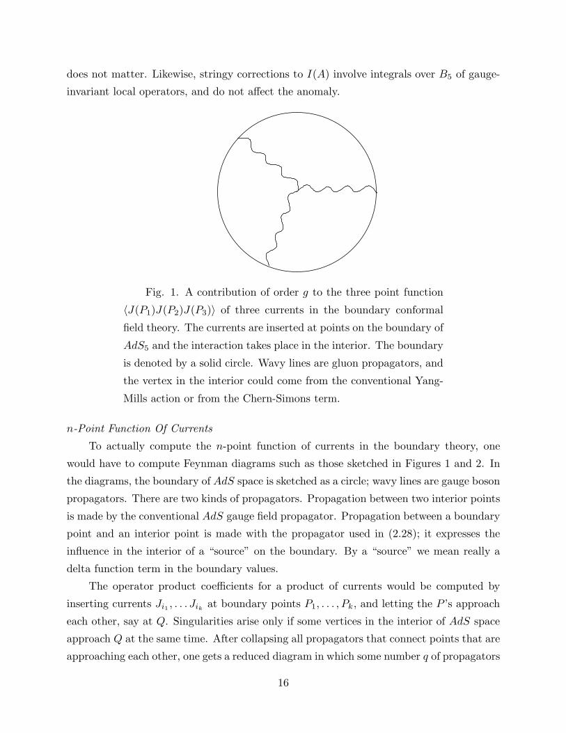
Fig. 1. A contribution of order g to the three point function

〈J(P1)J(P2)J(P3)〉 of three currents in the boundary conformal

field theory. The currents are inserted at points on the boundary of

AdS5 and the interaction takes place in the interior. The boundary

is denoted by a solid circle. Wavy lines are gluon propagators, and

the vertex in the interior could come from the conventional Yang-

Mills action or from the Chern-Simons term.

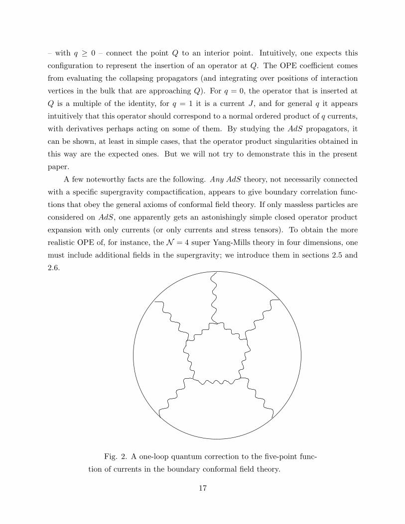
n-Point Function Of Currents

To actually compute the n-point function of currents in the boundary theory, one

would have to compute Feynman diagrams such as those sketched in Figures 1 and 2. In

the diagrams, the boundary of AdS space is sketched as a circle; wavy lines are gauge boson

propagators. There are two kinds of propagators. Propagation between two interior points

is made by the conventional AdS gauge field propagator. Propagation between a boundary

point and an interior point is made with the propagator used in (2.28); it expresses the

influence in the interior of a “source” on the boundary. By a “source” we mean really a

delta function term in the boundary values.

The operator product coefficients for a product of currents would be computed by

inserting currents Ji1 , . . . Jik at boundary points P1, . . . , Pk, and letting the P ’s approach

each other, say at Q. Singularities arise only if some vertices in the interior of AdS space

approach Q at the same time. After collapsing all propagators that connect points that are

approaching each other, one gets a reduced diagram in which some number q of propagators

16

– with q ≥ 0 – connect the point Q to an interior point. Intuitively, one expects this

configuration to represent the insertion of an operator at Q. The OPE coefficient comes

from evaluating the collapsing propagators (and integrating over positions of interaction

vertices in the bulk that are approaching Q). For q = 0, the operator that is inserted at

Q is a multiple of the identity, for q = 1 it is a current J , and for general q it appears

intuitively that this operator should correspond to a normal ordered product of q currents,

with derivatives perhaps acting on some of them. By studying the AdS propagators, it

can be shown, at least in simple cases, that the operator product singularities obtained in

this way are the expected ones. But we will not try to demonstrate this in the present

paper.

A few noteworthy facts are the following. Any AdS theory, not necessarily connected

with a specific supergravity compactification, appears to give boundary correlation func-

tions that obey the general axioms of conformal field theory. If only massless particles are

considered on AdS, one apparently gets an astonishingly simple closed operator product

expansion with only currents (or only currents and stress tensors). To obtain the more

realistic OPE of, for instance, the N = 4 super Yang-Mills theory in four dimensions, one

must include additional fields in the supergravity; we introduce them in sections 2.5 and

2.6.

Fig. 2. A one-loop quantum correction to the five-point func-

tion of currents in the boundary conformal field theory.

17

Gravity

Now we will discuss, though only schematically, the gravitational case, that is, the

dependence of the effective action of the boundary conformal field theory on the conformal

structure on the boundary. We consider a nonstandard conformal structure on Sd and

find, in accord with the Graham-Lee theorem, an Einstein metric on Bd+1 that induces

the given conformal structure on Sd. To compute the partition function of the conformal

field theory, we must evaluate the Einstein action on Bd+1 for this metric. In writing this

action, we must remember to include a surface term [50,51] in the Einstein action. The

action thus reads

I(g) =

∫

Bd+1

dd+1x√g

(1

2R+ Λ

)+

∫

∂Bd+1

K, (2.32)

where R is the scalar curvature, Λ the cosmological constant, and K is the trace of the

second fundamental form of the boundary.

Now, everything in sight in (2.32) is divergent. The Einstein equations Rij − 12gijR =

Λgij imply that R is a constant, so that the bulk integral in (2.32) is just a multiple of the

volume of Bd+1. This is of course infinite. Also, there is a question of exactly what the

boundary term in (2.32) is supposed to mean, if the boundary is at infinity. To proceed,

therefore, we need to regularize the action. The rough idea is to pick a positive function

f on Bd+1 that has a first order zero near the boundary. Of course, this breaks conformal

invariance on the boundary of Bd+1, and determines an actual metric h on Sd via (2.2).

We can regularize the volume integral by limiting it to the region B(ǫ) defined by f > ǫ.

Also, the boundary term in the action now gets a precise meaning: one integrates over the

boundary of B(ǫ). Of course, divergences will appear as ǫ→ 0.

We want to show at least schematically that, with a natural choice of f , the divergent

terms are local integrals on the boundary. The strategy for proving this is as follows.

Theorems 2.1 and 2.3 of [44] show that the metric of Bd+1 is determined locally by the

conformal structure of Sd up to very high order. The proof of the theorems in section 5

of that paper involves showing that once one picks a metric on Sd in its given conformal

class, one can pick distinguished coordinates near the boundary of Bd+1 to very high

order. These distinguished coordinates give a natural definition of f to high order and with

that definition, the divergent part of the action depends locally on the metric of Sd. The

divergent terms are thus local integrals on Sd, of the general form∫Sd d

dx√hP (R,∇R, . . .),

where P is a polynomial in the Riemann tensor of Sd and its derivatives.

18

The effective action of the conformal field theory on Sd can thus be made finite

by subtracting local counterterms. After the subtractions are made, the resulting finite

effective action will not necessarily be conformally invariant, but the conformal anomaly

– the variation of the effective action under conformal transformations of the metric – will

be given by a local expression. In fact, the conformal anomaly comes as usual from the

logarithmically divergent term; all the divergent terms are local.

The structure that we have described is just what one obtains when a conformal

field theory is coupled to a background metric. A regularization that breaks conformal

invariance is required. After picking a regularization, one encounters divergent terms which

are local; on subtracting them, one is left with a local conformal anomaly. The structure of

the conformal anomaly in general dimensions is reviewed in [52]. The conformal anomaly

arises only for even d; this is related to the fact that Theorems 2.1 and 2.3 in [44] make

different claims for odd and even d. In the even d case, the theorems allow logarithmic

terms that presumably lead to the conformal anomaly.

2.5. The Massive Case

We have come about as far as we can considering only massless fields on AdS space.

To really make contact with the ideas in [13] requires considering massive excitations as

well, since, among other reasons, the AdS compactifications considered in [13] apparently

do not have consistent low energy truncations in which only massless fields are included.

The reason for this last statement is that in, for instance, the AdS5 × S5 example, the

radius of the S5 is comparable to the radius of curvature of the AdS5, so that the inverse

radius of curvature (which behaves in AdS space roughly as the smallest wavelength of any

excitation, as seen in [24]) is comparable to the masses of the Kaluza-Klein excitations.

For orientation, we consider a scalar with mass m in AdSd+1. The action is

I(φ) =1

2

∫dµ(|dφ|2 +m2φ2

)(2.33)

with dµ the Riemannian measure. The wave equation, which we wrote before as (2.8),

receives an extra contribution from the mass term, and is now(− 1

(sinh y)dd

dy(sinh y)d

d

dy+

L2

sinh2 y+m2

)φ = 0. (2.34)

The L2 term is still irrelevant at large y. The two linearly independent solutions of (2.34)

behave for large y as eλy where

λ(λ+ d) = m2. (2.35)

19

For reasons that will be explained later, m2 is limited to the region in which this quadratic

equation has real roots. Let λ+ and λ− be the larger and smaller roots, respectively; note

that λ+ ≥ −d/2 and λ− ≤ −d/2. One linear combination of the two solutions extends

smoothly over the interior of AdSd+1; this solution behaves at infinity as exp(λ+y).

This state of affairs means that we cannot find a solution of the massive equation of

motion (2.34) that approaches a constant at infinity. The closest that we can do is the

following. Pick any positive function f on Bd+1 that has a simple zero on the boundary.

For instance, f could be e−y (which has a simple zero on the boundary, as one can see by

mapping back to the unit ball with r = tanh(y/2)). Then one can look for a solution of

the equation of motion that behaves as

φ ∼ f−λ+φ0, (2.36)

with an arbitrary “function” φ0 on the boundary.

But just what kind of object is φ0? The definition of φ0 as a function depends on the

choice of a particular f , which was the same choice used in (2.2) to define a metric (and

not just a conformal structure) on the boundary of AdSd+1. If we transform f → ewf ,

the metric will transform by ds2 → e2wds2. At the same time, (2.36) shows that φ0 will

transform by φ0 → ewλ+φ0. This transformation under conformal rescalings of the metric

shows that φ0 must be understood as a conformal density of length dimension λ+, or mass

dimension −λ+. (Henceforth, the word “dimension” will mean mass dimension.)

Computation Of Two Point Function

If, therefore, in a conformal field theory on the boundary of AdSd+1, there is a coupling∫φ0O for some operator O, then O must have conformal dimension d+ λ+. Let us verify

this by computing the two point function of the field O.

To begin with, we need to find the explicit form of a function φ that obeys the massive

wave equation and behaves as f−λ+φ0 at infinity. We represent AdS space as the half-

space x0 ≥ 0 with metric ds2 = (1/x20)(dx

20 +∑i dx

2i ). As before, the first step is to find a

Green’s function, that is a solution of (−DiDi+m2)K = 0 that vanishes on the boundary

except at one point. Again taking this point to be at x0 = ∞, K should be a function of

x0 only, and the equation reduces to

(−xd+1

0

d

dx0x−d+1

0

d

dx0+m2

)K(x0) = 0. (2.37)

20

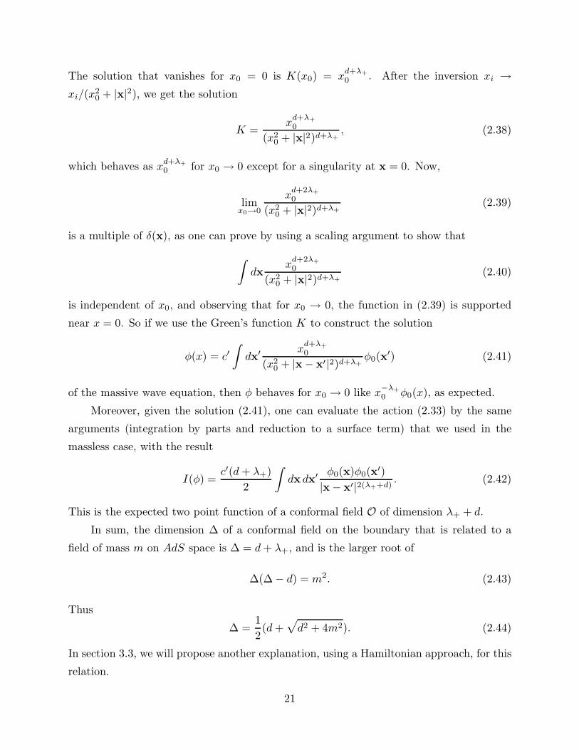
The solution that vanishes for x0 = 0 is K(x0) = xd+λ+

0 . After the inversion xi →xi/(x

20 + |x|2), we get the solution

K =xd+λ+

0

(x20 + |x|2)d+λ+

, (2.38)

which behaves as xd+λ+

0 for x0 → 0 except for a singularity at x = 0. Now,

limx0→0

xd+2λ+

0

(x20 + |x|2)d+λ+

(2.39)

is a multiple of δ(x), as one can prove by using a scaling argument to show that

∫dx

xd+2λ+

0

(x20 + |x|2)d+λ+

(2.40)

is independent of x0, and observing that for x0 → 0, the function in (2.39) is supported

near x = 0. So if we use the Green’s function K to construct the solution

φ(x) = c′∫dx′ x

d+λ+

0

(x20 + |x − x′|2)d+λ+

φ0(x′) (2.41)

of the massive wave equation, then φ behaves for x0 → 0 like x−λ+

0 φ0(x), as expected.

Moreover, given the solution (2.41), one can evaluate the action (2.33) by the same

arguments (integration by parts and reduction to a surface term) that we used in the

massless case, with the result

I(φ) =c′(d+ λ+)

2

∫dx dx′ φ0(x)φ0(x

′)

|x − x′|2(λ++d). (2.42)

This is the expected two point function of a conformal field O of dimension λ+ + d.

In sum, the dimension ∆ of a conformal field on the boundary that is related to a

field of mass m on AdS space is ∆ = d+ λ+, and is the larger root of

∆(∆ − d) = m2. (2.43)

Thus

∆ =1

2(d+

√d2 + 4m2). (2.44)

In section 3.3, we will propose another explanation, using a Hamiltonian approach, for this

relation.

21

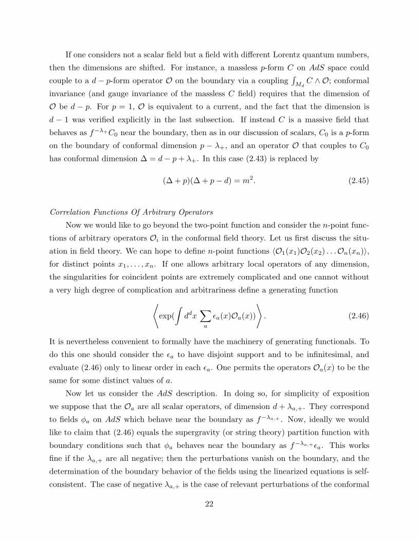
If one considers not a scalar field but a field with different Lorentz quantum numbers,

then the dimensions are shifted. For instance, a massless p-form C on AdS space could

couple to a d− p-form operator O on the boundary via a coupling∫Md

C ∧ O; conformal

invariance (and gauge invariance of the massless C field) requires that the dimension of

O be d − p. For p = 1, O is equivalent to a current, and the fact that the dimension is

d − 1 was verified explicitly in the last subsection. If instead C is a massive field that

behaves as f−λ+C0 near the boundary, then as in our discussion of scalars, C0 is a p-form

on the boundary of conformal dimension p − λ+, and an operator O that couples to C0

has conformal dimension ∆ = d− p+ λ+. In this case (2.43) is replaced by

(∆ + p)(∆ + p− d) = m2. (2.45)

Correlation Functions Of Arbitrary Operators

Now we would like to go beyond the two-point function and consider the n-point func-

tions of arbitrary operators Oi in the conformal field theory. Let us first discuss the situ-

ation in field theory. We can hope to define n-point functions 〈O1(x1)O2(x2) . . .On(xn)〉,for distinct points x1, . . . , xn. If one allows arbitrary local operators of any dimension,

the singularities for coincident points are extremely complicated and one cannot without

a very high degree of complication and arbitrariness define a generating function

⟨exp(

∫ddx

∑

a

ǫa(x)Oa(x))

⟩. (2.46)

It is nevertheless convenient to formally have the machinery of generating functionals. To

do this one should consider the ǫa to have disjoint support and to be infinitesimal, and

evaluate (2.46) only to linear order in each ǫa. One permits the operators Oa(x) to be the

same for some distinct values of a.

Now let us consider the AdS description. In doing so, for simplicity of exposition

we suppose that the Oa are all scalar operators, of dimension d+ λa,+. They correspond

to fields φa on AdS which behave near the boundary as f−λa,+ . Now, ideally we would

like to claim that (2.46) equals the supergravity (or string theory) partition function with

boundary conditions such that φa behaves near the boundary as f−λa,+ǫa. This works

fine if the λa,+ are all negative; then the perturbations vanish on the boundary, and the

determination of the boundary behavior of the fields using the linearized equations is self-

consistent. The case of negative λa,+ is the case of relevant perturbations of the conformal

22

field theory, of dimension < d, and it should come as no surprise that this is the most

favorable case for defining the functional (2.46) as an honest functional of the ǫa (and not

just for infinitesimal ǫa). One can also extend this to include operators with vanishing

λa,+, corresponding to marginal perturbations of the conformal field theory. For this,

one must go beyond the linearized approximation in describing the boundary fields, and

include general boundary values of massless fields, which we introduced in section 2.3.

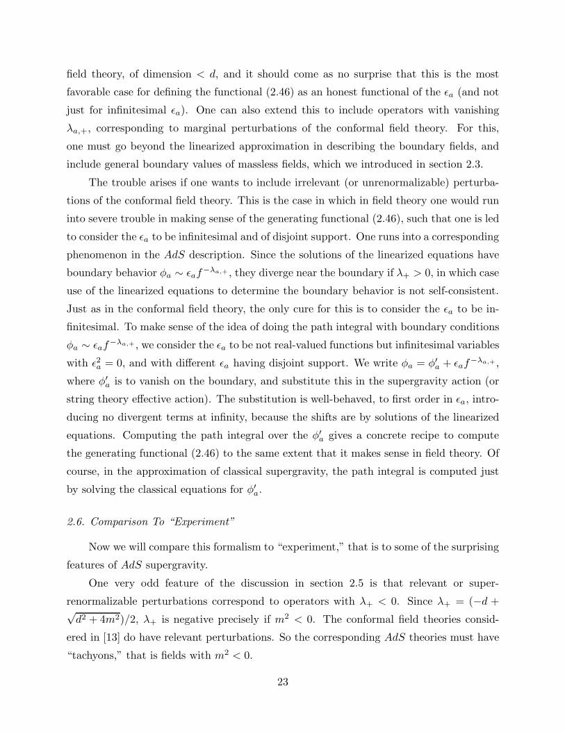
The trouble arises if one wants to include irrelevant (or unrenormalizable) perturba-

tions of the conformal field theory. This is the case in which in field theory one would run

into severe trouble in making sense of the generating functional (2.46), such that one is led

to consider the ǫa to be infinitesimal and of disjoint support. One runs into a corresponding

phenomenon in the AdS description. Since the solutions of the linearized equations have

boundary behavior φa ∼ ǫaf−λa,+ , they diverge near the boundary if λ+ > 0, in which case

use of the linearized equations to determine the boundary behavior is not self-consistent.

Just as in the conformal field theory, the only cure for this is to consider the ǫa to be in-

finitesimal. To make sense of the idea of doing the path integral with boundary conditions

φa ∼ ǫaf−λa,+ , we consider the ǫa to be not real-valued functions but infinitesimal variables

with ǫ2a = 0, and with different ǫa having disjoint support. We write φa = φ′a + ǫaf−λa,+ ,

where φ′a is to vanish on the boundary, and substitute this in the supergravity action (or

string theory effective action). The substitution is well-behaved, to first order in ǫa, intro-

ducing no divergent terms at infinity, because the shifts are by solutions of the linearized

equations. Computing the path integral over the φ′a gives a concrete recipe to compute

the generating functional (2.46) to the same extent that it makes sense in field theory. Of

course, in the approximation of classical supergravity, the path integral is computed just

by solving the classical equations for φ′a.

2.6. Comparison To “Experiment”

Now we will compare this formalism to “experiment,” that is to some of the surprising

features of AdS supergravity.

One very odd feature of the discussion in section 2.5 is that relevant or super-

renormalizable perturbations correspond to operators with λ+ < 0. Since λ+ = (−d +√d2 + 4m2)/2, λ+ is negative precisely if m2 < 0. The conformal field theories consid-

ered in [13] do have relevant perturbations. So the corresponding AdS theories must have

“tachyons,” that is fields with m2 < 0.

23

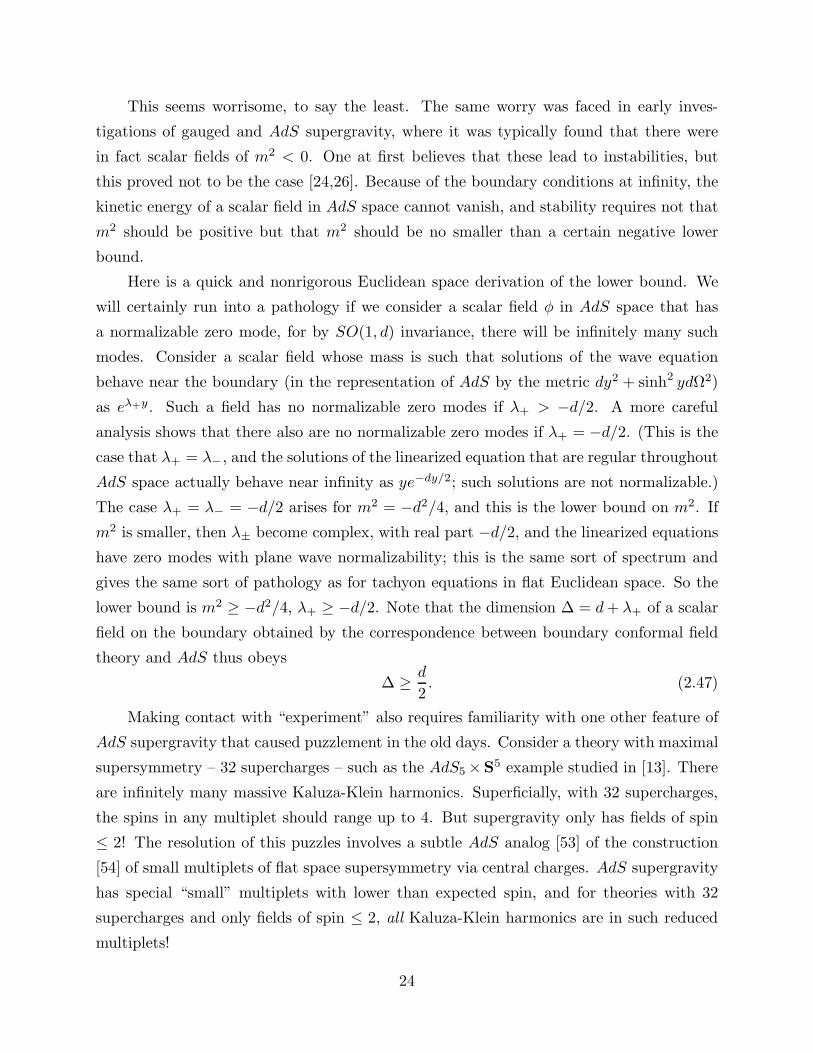
This seems worrisome, to say the least. The same worry was faced in early inves-

tigations of gauged and AdS supergravity, where it was typically found that there were

in fact scalar fields of m2 < 0. One at first believes that these lead to instabilities, but

this proved not to be the case [24,26]. Because of the boundary conditions at infinity, the

kinetic energy of a scalar field in AdS space cannot vanish, and stability requires not that

m2 should be positive but that m2 should be no smaller than a certain negative lower

bound.

Here is a quick and nonrigorous Euclidean space derivation of the lower bound. We

will certainly run into a pathology if we consider a scalar field φ in AdS space that has

a normalizable zero mode, for by SO(1, d) invariance, there will be infinitely many such

modes. Consider a scalar field whose mass is such that solutions of the wave equation

behave near the boundary (in the representation of AdS by the metric dy2 + sinh2 ydΩ2)

as eλ+y. Such a field has no normalizable zero modes if λ+ > −d/2. A more careful

analysis shows that there also are no normalizable zero modes if λ+ = −d/2. (This is the

case that λ+ = λ−, and the solutions of the linearized equation that are regular throughout

AdS space actually behave near infinity as ye−dy/2; such solutions are not normalizable.)

The case λ+ = λ− = −d/2 arises for m2 = −d2/4, and this is the lower bound on m2. If

m2 is smaller, then λ± become complex, with real part −d/2, and the linearized equations

have zero modes with plane wave normalizability; this is the same sort of spectrum and

gives the same sort of pathology as for tachyon equations in flat Euclidean space. So the

lower bound is m2 ≥ −d2/4, λ+ ≥ −d/2. Note that the dimension ∆ = d+ λ+ of a scalar

field on the boundary obtained by the correspondence between boundary conformal field

theory and AdS thus obeys

∆ ≥ d

2. (2.47)

Making contact with “experiment” also requires familiarity with one other feature of

AdS supergravity that caused puzzlement in the old days. Consider a theory with maximal

supersymmetry – 32 supercharges – such as the AdS5 ×S5 example studied in [13]. There

are infinitely many massive Kaluza-Klein harmonics. Superficially, with 32 supercharges,

the spins in any multiplet should range up to 4. But supergravity only has fields of spin

≤ 2! The resolution of this puzzles involves a subtle AdS analog [53] of the construction

[54] of small multiplets of flat space supersymmetry via central charges. AdS supergravity

has special “small” multiplets with lower than expected spin, and for theories with 32

supercharges and only fields of spin ≤ 2, all Kaluza-Klein harmonics are in such reduced

multiplets!

24

The Kaluza-Klein harmonics are important in the present discussion for the following

reason. In the models considered in [13], in a limit in which classical supergravity is valid,

the states with masses of order one are precisely the Kaluza-Klein modes. Indeed, in for

example the AdS5×S5 model, the radius of the S5 is comparable to the radius of curvature

of the AdS5 factor, so the Kaluza-Klein harmonics have masses of order one, in units of the

AdS5 length scale. Stringy excitations are much heavier; for instance, in this model they

have masses of order (g2YMN)1/4 (which is large in the limit in which classical supergravity

is valid), as shown in [13].

Since the dimension of a scalar operator in the four-dimensional conformal field theory

is

∆ = d+ λ+ =d+

√d2 + 4m2

2, (2.48)

the particles of very large mass inAdS space correspond to operators of very high dimension

in the conformal field theory. The conformal fields with dimensions of order one correspond

therefore precisely to the Kaluza-Klein excitations.

Since the Kaluza-Klein excitations are in “small” representations of supersymme-

try, their masses are protected against quantum and stringy corrections. The conformal

fields that correspond to these excitations are similarly in “small” representations, with

dimensions that are protected against quantum corrections. It is therefore possible to

test the conjectured CFT/AdS correspondence by comparing the Kaluza-Klein harmonics

on AdS5 × S5 to the operators in the N = 4 super Yang-Mills theory that are in small

representations of supersymmetry; those operators are discussed in [55].

The Kaluza-Klein harmonics have been completely worked out in [30,31]. The oper-

ators of spin zero are in five infinite families. We will make the comparison to the N = 4

theory for the three families that contain relevant or marginal operators. Two additional

families that contain only states of positive m2 will not be considered here.

We recall the following facts about the N = 4 theory. This theory has an R-symmetry

group SU(4), which is a cover of SO(6). Viewed as an N = 0 theory, it has six real scalars

Xa in the 6 or vector of SO(6) and adjoint represention of the gauge group, and four

fermions λAα , also in the adjoint representation of the gauge group, in the 4 of SU(4)

or positive chirality spinor of SO(6). (Here a = 1, . . . , 6 is a vector index of SO(6), A =

1, . . . , 4 is a positive chirality SO(6) spinor index, and α is a positive chirality Lorentz spinor

index.) From the point of view of an N = 1 subalgebra of the supersymmetry algebra,

this theory has three chiral superfields Φz, z = 1, . . . , 3 in the adjoint representation, and

25

a chiral superfield Wα, also in the adjoint representation, that contains the gauge field

strength. The superpotential is W = ǫz1z2z3TrΦz1 [Φz2 ,Φz3 ]. Viewed as an N = 2 theory,

this theory has a vector multiplet and a hypermultiplet in the adjoint representation.

We can now identify the following families of operators in the N = 4 theory that are

in small representations:

(1) First we view the theory from an N = 1 point of view. Any gauge-invariant

polynomial in chiral superfields is a chiral operator. If it is not a descendant, that is it

cannot be written in the form Qα,Λα for any Λα, then it is in a “small” representation

of supersymmetry. Consider the operators T z1z2...zk = TrΦz1Φz2 . . .Φzk . We require k ≥ 2

as the gauge group is SU(N) and not U(N). If one symmetrizes in z1, . . . , zk, one gets

chiral fields that are in “small” representations. If one does not so symmetrize, one gets

a descendant, because of the fact that the commutators [Φzi ,Φzj ] are derivatives of the

superpotential W .

From the N = 1 point of view, the theory has a U(3) global symmetry, of which the

U(1) acts as a group of R-symmetries. The R-charge of T z1z2...zk is k times that of Φ. The

operator T z1z2...zk has dimension k in free field theory. Its dimension is determined by the

R-charge and so is exactly k, for all values of the coupling. From a U(3) point of view, T

transforms in the representation which is the k-fold symmetric product of the 3 with itself.

Restoring the SO(6) symmetry of the N = 4 theory, this U(3) representation is part of the

SO(6) representation containing symmetric traceless tensors T a1a2...ak of order k. A field

of dimension k in four-dimensional conformal field theory has λ+ = k− 4 and corresponds

to a scalar field in supergravity with a mass m2 = λ+(λ+ + 4) = k(k − 4). So we expect

in the Kaluza-Klein spectrum of the N = 4 theory that for every k = 2, 3, . . . there should

be a scalar with mass m2 = k(k − 4) transforming in the kth traceless symmetric tensor

representation of SO(6). These states can be found in eqn. (2.34) and in Fig. 2 and Table

III of [30]. (Formulas given there contain a parameter e which we have set to 1.) Note that

a k = 1 state does not appear in the supergravity, which confirms that the supergravity

is dual to an SU(N) gauge theory and not to a U(N) theory.7 In fact, the k = 2 state

saturates the bound (2.47), and a k = 1 state would violate it. For k = 2 we get the

7 Another reason that the U(1) gauge field could not be coded in the AdS5 theory is that it

is free, while in the AdS5 theory everything couples to gravity and nothing is free. To describe

U(N) gauge theory on the boundary, one would have to supplement the AdS5 theory with an

explicit U(1) singleton field on the boundary.

26

relevant operator TrXaXb − (1/6)δabTrX2 (however, the operator∑a Tr(Xa)2, which is

certainly a relevant operator for weak coupling, is not chiral and so is related to a stringy

excitation and has a dimension of order (g2YMN)1/4 for strong coupling).

(2) Likewise, we can make the chiral superfield V z1...zt = TrWαWαΦz1Φz2 . . .Φzt for

t ≥ 0. Again, modulo descendants one can symmetrize in the ordering of all t+ 2 factors.

These operators have dimension t + 3 in free field theory, and again their dimensions are

protected by theR-symmetry. If we set t = 0, we get the relevant operator TrWαWα, which

is a linear combination of the gluino bilinears TrλAαλαB , which transform in the 10 of SO(6)

(one can think of this representation as consisting of self-dual third rank antisymmetric

tensors). For higher t, these states transform in the representation obtained by tensoring

the 10 with the tth rank symmetric tensors and removing traces. Setting k = t + 1, we

hence expect for k = 1, 2, 3, . . . a supergravity harmonic in the representation just stated

with mass

m2 = (k + 2)(k − 2). (2.49)

Such a harmonic is listed in Fig. 2 and in Table III in [30].

(3) The conformal field theory also contains a special marginal operator, the deriva-

tive of the Lagrangian density with respect to the Yang-Mills coupling. This operator is

in a small representation, since the Lagrangian cannot be written as an integral over a

superspace with 16 fermionic coordinates. It transforms in the singlet representation of

SO(6), and, being a marginal operator, is related to a supergravity mode with m2 = 0,

in fact, the dilaton. To exhibit this operator as the first in an infinite series, view the

N = 4 theory as an N = 2 theory with a vector multiplet and an adjoint hypermultiplet.

Let a be the complex scalar in the vector multiplet. Possible Lagrangians for the vector

multiplets, with N = 2 supersymmetry and the smallest possible number of derivatives,

are determined by a “prepotential,” which is a holomorphic, gauge-invariant function of

a. A term Tr ar in the prepotential leads to an operator Qr = Tr ar−2 FijFij + . . . which

could be added to the Lagrangian density while preserving N = 2 supersymmetry. These

operators are all in small representations as the couplings coming from the prepotential

cannot be obtained by integration over all of N = 2 superspace. Qr has dimension 2 + r

in free field theory, and this dimension is protected by supersymmetry. Since a is part of

a vector of SO(6), Qr is part of a set of operators transforming in the r − 2th symmetric

tensor representation of SO(6). (In fact, Qr can be viewed as a highest weight vector for

this representation.) Hence, if we set k = r−2, we have for k ≥ 0 an operator of dimension

27

k+4 in the kth symmetric tensor representation, corresponding to Kaluza-Klein harmonics

in that representation with mass

m2 = k(k + 4). (2.50)

These states can be found in Fig. 2 and Table III in [30].

3. Other Spacetimes And Hamiltonian Formalism

3.1. General Formalism

The CFT-AdS correspondence relates conformal field theory on Sd to supergravity on

AdSd+1 ×W , where W is a compact manifold (a sphere in the maximally supersymmetric

cases). What happens if we replace Sd by a more general compact d-manifold N? The

natural intuitive answer is that one should then replace AdSd+1 by a d + 1-dimensional

Einstein manifold X with negative cosmological constant. The relation between X and M

should be just like the relation between Sd and AdSd+1. X should have a compactification

consisting of a manifold with boundary X, whose boundary points are M and whose

interior points are X , and such that the metric on X has a double pole near the boundary.

Then the metric on X determines a conformal structure on M , just as we reviewed in

section 2.1 in the case of AdSd+1 and Sd.

More generally, instead of a d+1-manifoldX , one might use a manifold Y of dimension

10 or 11 (depending on whether one is doing string theory or M -theory) that looks near

infinity like X ×W for some Einstein manifold X . Moreover, Y might contain various

branes or stringy impurities of some kind. These generalizations are probably necessary,

since M might be, for example, a four-manifold of non-zero signature, which is not the

boundary of any five-manifold. (However, it may be that for such M ’s, the conformal field

theory partition function diverges for reasons discussed at the end of section 2.3.) But

since the discussion is non-rigorous anyway, we will keep things simple and speak in terms

of a d+ 1-dimensional Einstein manifold X .

Once X is found, how will we use it to study conformal field theory on M? As in

section 2.3, we propose that the conformal field theory partition function on M equals the

supergravity (or string theory) partition function on X , with boundary conditions given by

the conformal structure (and other fields) on M . In the approximation of classical super-

gravity, we simply solve the classical equations on X with the given boundary conditions,

and write

ZCFT (M) = exp(−IS(X)), (3.1)

28

where ZCFT (M) is the conformal field theory partition function on M and IS is the

supergravity action.

In general, there might be several possible X ’s. If so, we have no natural way to pick

one, so as is usual in Euclidean quantum gravity, we replace (3.1) by a sum. Before writing

the sum, it is helpful to note that in the large N limit, IS(X) is proportional to a positive

power of N , in fact IS = NγF (X) for some γ > 0. For example, γ = 2 for N = 4 super

Yang-Mills in four dimensions. So we postulate that in general

ZCFT (M) =∑

i

exp(−NγF (Xi)), (3.2)

where the Xi are the Einstein manifolds of boundary M .

Another refinement involves spin structures. M may admit several spin structures, in

which case ZCFT (M) will in general depend on the spin structure on M . If so, we select

a spin structure on M and restrict the sum in (3.2) to run over those Xi over which the

given spin structure on M can be extended. 8

Of course, (3.2) should be viewed as the classical supergravity approximation to an

an exact formula

ZCFT (M) =∑

i

ZS(Xi), (3.3)

where ZS(Xi) is the partition function of string theory on Xi.

Now, as M is compact, there are no conventional phase transitions in evaluating path

integrals on M . As long as ZCFT (M) is sufficiently convergent (we discussed obstructions

to convergence at the end of section 2.3), ZCFT (M) is a smooth function of the conformal

structure of M (and other fields on M). However, in (3.2) we see a natural mechanism for

a singularity or phase transition that would arise only in the large N limit. In the large

N limit, the sum in (3.2) will be dominated by that Xi for which F (Xi) is smallest. If

F (M) = − lnZCFT (M) is the conformal field theory free energy, then

limN→∞

F (M)

Nγ= F (Xi), (3.4)

8 There may be further refinements of a similar nature. For example, in the case that the

boundary theory is four-dimensional gauge theory with a gauge group that is locally SU(N), it

may be that the gauge group is really SU(N)/ZN , in which case the partition function on M

depends on a choice of a “discrete magnetic flux” w ∈ H2(M,Z). Perhaps one should restrict the

sum in (3.2) to Xi over which w extends.

29

for that value of i for which F (Xi) is least. At a point at which F (Xi) = F (Xj) for some

i 6= j, one may well “jump” from one branch to another. This will produce a singularity

of the large N theory, somewhat similar to large N singularities found [47] in certain toy

models.

3.2. A Concrete Example

We will next describe a concrete example, namely M = S1 × Sd−1, in which one

can explicitly describe two possible X ’s and a transition between them. In fact, the two

solutions were described (in the four-dimensional case) by Hawking and Page [56] who also

pointed out the existence of the phase transition (which they of course interpreted in terms

of quantum gravity rather than boundary conformal field theory!).

The first solution is obtained as follows. The simplest way to find Einstein manifolds

is to take the quotient of a portion of AdSd+1 by a group that acts discretely on it. AdSd+1

can be described as the quadric

uv −d∑

i=1

x2i = 1. (3.5)

(The analogous formula for AdSd+1 with Lorentz signature is given in (1.2).) We restrict

ourselves to the region AdS+d+1 of AdS space with u, v > 0. We consider the action on

AdS+d+1 of a group Z generated by the transformation

u→ λ−1u, v → λv, xi → xi, (3.6)

with λ a fixed real number greater than 1. This group acts freely on AdS+d+1. Let X1 be

the quotient X1 = AdS+d+1/Z. To describe X1, we note that a fundamental domain for

the action of Z on v is 1 ≤ v ≤ λ, with v = 1 and v = λ identified. v parametrizes a circle,

on which a natural angular coordinate is

θ = 2π ln v/ lnλ. (3.7)

For given v, one can solve for u by u = (1 +∑i x

2i )/v. So X1 is spanned by xi and θ, and

is topologically R4 × S1. To see what lies at “infinity” in X1, we drop the 1 in (3.5), to

get

uv −d∑

i=1

x2i = 0, (3.8)

30

and regard u, v, and the xi as homogeneous coordinates, subject to a scaling relation

u → su, v → sv, xi → sxi with real positive s (s should be positive since we are working

in the region u, v > 0). (3.8) does not permit the xi to all vanish (since u, v > 0), so

one can use the scaling relation to set∑d

i=1 x2i = 1. The xi modulo the scaling relation

thus define a point in Sd−1. Just as before, v modulo the action of (3.6) defines a point

in S1, and one can uniquely solve (3.8) for u. Hence the boundary of X1 is a copy of

M = S1 × Sd−1.

An important property of this example is that it is invariant under an action of

SO(2)×SO(d). Here, SO(d) is the rotation group of the second factor in M = S1 ×Sd−1;

it acts by rotation of the xi in (3.5). SO(2) acts by rotation of the angle θ defined in (3.7).

The SO(2) × SO(d) symmetry uniquely determines the conformal structure of S1 × Sd−1

up to a constant β = lnλ which one can think of as the ratio of the radius of S1 to the

radius of Sd−1. M = S1 × Sd−1 has two spin structures – spinors may be periodic or

antiperiodic around the S1. The partition functions of M with these spin structures can

be interpreted respectively as

Z1(M) = Tr e−βH(−1)F (3.9)

or

Z2(M) = Tr e−βH . (3.10)

Here H is the Hamiltonian that generates time translations if one quantizes on Sd−1 × R

(with R as the “time” direction); or it is the dilation generator if the theory is formulated

on Rd. Note that Z1(M) is not really a supersymmetric index, at least not in a naive sense,

since compactification on Sd−1 breaks supersymmetry, that is, the dilation generator H

does not commute with any supersymmetries.

Both spin structures extend over X1, so X1 contributes to both Tr e−βH(−1)F and

Tr e−βH in the conformal field theory. Its contribution is, however, extremely simple in the

approximation of classical supergravity. The reason is that X1 = S1 × Rd, and β enters

only as the radius of S1. This ensures that the supergravity action is linear in β,

IS(X1) = βE (3.11)

for some constant E, since IS(X1) is computed from a local integral onX1 (plus a boundary

term that is a local integral at infinity), and β only enters in determining how far one

must integrate in the S1 direction. If one introduces additional background fields on

31

M = S1 × Sd−1 in a way that preserves the time-translation invariance of S1 × Sd−1,

then E may depend on the background fields, but is still independent of β. E should be

interpreted as the ground state energy in quantization of the conformal field theory on

Sd−1.

If we set r2 =∑i x

2i ,∑i(dxi)

2 = (dr)2+r2dΩ2, t = ln v+ 12 ln(1+r2), then the metric

of X1, which is just the AdS metric −du dv +∑i(dxi)

2 with some global identifications,

becomes

ds2 = (1 + r2)(dt)2 +(dr)2

1 + r2+ r2dΩ2, (3.12)

which is the form in which it is written in [56].

The Schwarzschild Solution

The second solution X2 is the AdS Schwarzschild solution. Topologically X2 = R2 ×Sd−1. The S1 factor in M = S1 × Sd−1 is the boundary (in a sense with which we are

by now familiar) of the R2 factor in X2. Being simply-connected, X2 has a unique spin

structure, which restricts on S1 to the antiperiodic spin structure. (This amounts to the

familiar fact in superstring theory that the antiperiodic or Neveu-Schwarz spin structure

on a circle is the one that extends over a disc.) Hence X2 contributes to Tr e−βH , but

not to Tr e−βH(−1)F . Hence Tr e−βH , but not Tr e−βH(−1)F , may have a large N phase

transition from a “flop” between X1 and X2. That it does, at least for d + 1 = 4, is

equivalent to facts described by Hawking and Page [56].

The metric of a Euclidean AdSd+1 Schwarzschild black hole of mass m, for d = 3, as

described in [56], eqn. 2.1, is

ds2 = V (dt)2 + V −1(dr)2 + r2dΩ2 (3.13)

with dΩ2 the line element on a round two-sphere, and

V = 1 − 2m

r+ r2. (3.14)

(Notation compares to that in [56] as follows: we set b = 1, since the form of the AdS

metric that we have used corresponds for AdS4 to Λ = −3; we set mp = 1, and write m

instead of M for the black hole mass.) Let r+ be the largest root of the equation V (r) = 0.

The spacetime is limited to the region r ≥ r+. The metric is smooth and complete if t is

regarded as an angular variable with period

β =12πr+1 + 3r2+

. (3.15)

32

This has a maximum as a function of r+, so the black hole spacetime X2 contributes to

the thermodynamics only for sufficiently small β, that is sufficiently large temperature.

The action difference between X2 and X1 was computed by Hawking and Page to be

I =πr2+(1 − r2+)

1 + 3r2+. (3.16)

This is negative for sufficiently large r+, that is for sufficiently small β or sufficiently large

temperature. Thus (for d = 3 and presumably for all d), the boundary conformal field

theories that enter the CFT-AdS correspondence have phase transitions as a function of

temperature in the large N limit.

Further support for the interpretation of the AdS black hole in terms of conformal field

theory at high temperature comes from the fact that the AdS black hole has positive specific

heat [56] in the region in which it has lower action. This is needed for the correspondence

with conformal field theory (which certainly has positive specific heat), and is a somewhat

surprising result, as it does not hold for Schwarzschild black holes in asymptotically flat

space.

On the other hand, it is also shown in [56] that very low mass AdS black holes have

negative specific heat, like black holes in asymptotically flat space. In fact, very small

mass black holes have a size much less than the AdS radius of curvature, and are very

similar to flat space black holes. Such black holes should decay by emission of Hawking

radiation; the CFT/AdS correspondence gives apparently a completely unitary, quantum

mechanical description of their decay.

Comparison With Gauge Theory Expectations

We will now specialize to the AdS5 × S5 case, and compare to the expected large N

behavior of four-dimensional gauge theories.

Actually, we do not know how the N = 4 theory should behave for large N with large

and fixed g2YMN . We will therefore compare to the expected large N thermodynamics [57]

of an SU(N) gauge theory with massive quarks in the fundamental representation (that

is, ordinary QCD generalized to large N). It is surprising that this comparison will work,

since QCD is confining, while the N = 4 theory has no obviously analogous phenomenon.

However, the comparison seems to work, as we will see, at least for large g2YMN .

The whole idea of the 1/N expansion as an approach to QCD [1] is that for large

N , the Hilbert space of the theory consists of color singlet particles whose masses and

33

multiplicities are independent of N . Suppose we formulate the theory on some three-

manifold K and define Z(β) = Tr e−βH , and F = − lnZ. The ground state energy E in

this theory is of order N2 (as vacuum diagrams receive contributions from N2 species of

gluon), while excitation energies and multiplicities are of order one. Hence, we expect that

limN→∞

F (β)

N2= β

E

N2. (3.17)

The idea is that as the excitations have multiplicity of order one, they contribute to F an

amount of order one, and make a vanishing contribution to the largeN limit of F/N2, which

hence should simply measure the ground state energy. The formula in (3.17) precisely has

the structure of the contribution (3.11) of the manifold X1 to the free energy.

In large N QCD, such behavior cannot prevail at all temperatures. At sufficiently high

temperatures, one “sees” that the theory is made of quarks and gluons. By asymptotic

freedom, the gluons are effectively free at high temperatures. As the number of species is of

order N2, they contribute to the free energy an amount of order N2, with a temperature

dependence determined by 3 + 1-dimensional conformal invariance. So for high enough

temperature, limN→∞(F (β)/N2) ∼ T 4 = β−4.

This behavior is precisely analogous to what we have found for the large N behavior

of the N = 4 theory. The low temperature phase, in which the N2 term in the free energy

is trivial (as it reflects only the contribution of the ground state), corresponds to the phase

in which the manifold X1 dominates. The high temperature phase, with a non-trivial N2

term in the free energy, corresponds to the phase in which the manifold X2 dominates.

3.3. Hamiltonian Interpretation

Our remaining goal will be to develop a Hamiltonian version of the CFT-AdS cor-

respondence and to use it to give another explanation of the relation between masses on

AdS space and conformal dimensions on the boundary theory.

We would like to describe in terms of supergravity the Hilbert space of the boundary

conformal field theory on Sd−1. The partition function of the conformal field theory on

S1 × Sd−1 can be computed in terms of the states obtained by quantizing on Sd−1. We

want the Hilbert space relevant to the low temperature phase – the low-lying excitations

of the large N vacuum. So we must compare the conformal field theory to the manifold

X1 = S1×Rd. We recall that X1 is just AdS with some global identifications, with metric

found in (3.12):

ds2 = (1 + r2)(dt)2 +(dr)2

1 + r2+ r2dΩ2. (3.18)

34

A t = 0 slice of X1 is a copy of Rd which can be regarded as an initial value hypersurface

in AdSd+1. The Hilbert space obtained by quantization on this t = 0 slice is hence simply

the quantum Hilbert space of the theory on AdSd+1.

So we identify the Hilbert space of the conformal field theory in quantization on Sd−1

with the Hilbert space of the supergravity (or string theory) on AdSd+1.

Now, in conformal field theory in d dimensions, the Hilbert space on Sd−1 has an

important interpretation, which is particularly well-known in the d = 2 case. Consider

formulating the theory on Rd and inserting an operator O at a point in Rd, say the origin.

Think of Sd−1 as a sphere around the origin. The path integral in the interior of the sphere

determines a quantum state |ψO〉 on the boundary, that is on Sd−1. Conversely, suppose

we are given a quantum state |ψ〉 on Sd−1. Given the conformal invariance, the overall

size of the Sd−1 does not matter. So we cut out a tiny hole around the origin, whose

boundary is a sphere of radius ǫ, and use the state |ψ〉 to define boundary conditions on

the boundary. In the limit as ǫ → 0, this procedure defines a local operator Oψ as seen

by an outside observer. These two operations are inverses of each other and give a natural

correspondence in conformal field theory between states on Sd−1 and local operators.

So we can assert that, in the CFT-AdS correspondence, the local operators in the

boundary conformal field theory correspond to the quantum states on AdSd+1.

As an application of this, we will recover the relation claimed in section 2.5 between

dimensions of operators in conformal field theory and particle masses on AdS space. Choos-

ing a point at the origin in Rd breaks the Euclidean signature conformal group SO(1, d+1)

to a subgroup that contains SO(1, 1) × SO(d). SO(d) is the group of rotations around

the given point, and SO(1, 1) is the group of dilatations. The SO(1, 1) eigenvalue is the

dimension of an operator. When the AdS metric is written as in (3.18), an SO(d) group

(which rotates the sphere whose line element is dΩ2) is manifest, and commutes with the

symmetry of time translations. We call the generator of time translations the energy. The

SO(1, 1) generator that measures operator dimensions in the conformal field theory is the

unique SO(1, d+ 1) generator that commutes with SO(d), so it is the energy operator of

the AdS theory.

Thus, the energy of a mode in AdS space equals the dimension of the corresponding

operator in the boundary conformal field theory. Now, in equation (A6) in [24], it is shown

that a scalar field of mass m2 in AdS space has a discrete energy spectrum (with the

definition of energy that we have just given), and that the frequency of the mode of lowest

energy is ω = 12 (d +

√d2 − 4m2). Comparing to the formula (2.44) for the dimension ∆

35

of the conformal field O in boundary conformal field theory that is related to a scalar of

mass m in AdS space, we see that ∆ = ω, as expected. 9 The same equation (A6) also

shows that the energies of excited modes of the massive field are of the form ω + integer,

and so agree with the dimensions of derivatives of O.

This work was supported in part by NSF Grant PHY-9513835. I am grateful to

N. Seiberg for many very helpful comments, to G. Tian for pointing out the work of

Graham and Lee, and to D. Freedman and P. van Nieuwenhuyzen for discussions of gauged

supergravity.

9 In [24], the computation is performed only for d = 3. Also, the parameter α in [24] is our

−m2, and there is a small clash in notation: the quantity λ+ defined on p. 276 of [24] is d + λ+

in our notation.

36

References

[1] G. ’t Hooft, “A Planar Diagram Theory For Strong Interactions,” Nucl. Phys. B72

(1974) 461.

[2] A. M. Polyakov, “String Theory And Quark Confinement,” hep-th/9711002.

[3] G. Gibbons, Nucl. Phys. B207 (1982) 337; R. Kallosh and A. Peet, Phys. Rev. B46

(1992) 5223, hep-th/9209116; S. Ferrara, G. Gibbons, R. Kallosh, Nucl. Phys. B500

(1997) 75, hep-th/9702103.

[4] G. Gibbons and P. Townsend, “Vacuum Interpolation In Supergravity Via Super p-

Branes,” Phys. Rev. Lett. 71 (1993) 5223.

[5] M. J. Duff, G. W. Gibbons, and P. K. Townsend, “Macroscopic Superstrings As In-

terpolating Solitons,” Phys. Lett. B332 (1994) 321.

[6] G. W. Gibbons, G. T. Horowitz, and P. K. Townsend, “Higher Dimensional Resolution

Of Dilatonic Black Hole Singularities,” Class. Quant. Grav. 12 (1995) 297.

[7] S. Ferrara, G. W. Gibbons, and R. Kallosh, “Black Holes And Critical Points In Moduli

Space,” Nucl. Phys. B500 (1997) 75, hep-th/9702103; A. Chamseddine, S. Ferrara,

G. W. Gibbons, and R. Kallosh, “Enhancement Of Supersymmetry Near 5−D Black

Hole Horizon,” Phys. Rev. D55 (1997) 3647, hep-th/9610155.

[8] S. S. Gubser, I. R. Klebanov, and A. W. Peet, “Entropy And Temperature Of Black

3-Branes,” Phys. Rev. D54 (1996) 3915.

[9] I. R. Klebanov, “World Volume Approach To Absorption By Nondilatonic Branes,”

Nucl. Phys. B496 (1997) 231.

[10] S. S. Gubser, I. R. Klebanov, A. A. Tseytlin, “String Theory And Classical Absorption

By Three-branes,” Nucl. Phys. B499 (1997) 217.

[11] S. S. Gubser and I. R. Klebanov, “Absorption By Branes And Schwinger Terms In

The World Volume Theory,” Phys. Lett. B413 (1997) 41.

[12] J. Maldacena and A. Strominger, “Semiclassical Decay Of Near Extremal Fivebranes,”

hep-th/9710014.

[13] J. Maldacena, “The Large N Limit Of Superconformal Field Theories And Super-

gravity,” hep-th/971120.

[14] N. Itzhaki, J. M. Maldacena, J. Sonnenschein, and S. Yankielowicz, “Supergravity

And The Large N Limit Of Theories With Sixteen Supercharges,” hep-th/9802042.

[15] S. Hyun, “U -Duality Between Three And Higher Dimensional Black Holes,” hep-

th/9704005; S. Hyun, Y. Kiem, and H. Shin, “Infinite Lorentz Boost Along The

M Theory Circle And Nonasymptotically Flat Solutions In Supergravities,” hep-

th/9712021.

[16] K. Sfetsos and K. Skenderis, “Microscopic Derivation Of The Bekenstein-Hawking

Entropy Formula For Nonextremal Black Holes,” hep-th/9711138; H. J. Boonstra, B.

Peeters, and K. Skenderis, “Branes And Anti-de Sitter Space-times,” hep-th/9801076.

37

[17] P. Claus, R. Kallosh, and A. van Proeyen, “M Five-brane And Superconformal (0, 2)

Tensor Multiplet In Six-Dimensions,” hep-th/9711161; P. Claus, R. Kallosh, J. Kumar,

P. Townsend, and A. van Proeyen, “Conformal Theory Of M2, D3, M5, and D1-

Branes + D5-Branes,” hep-th/9801206.

[18] R. Kallosh, J. Kumar, and A. Rajaraman, “Special Conformal Symmetry Of

W0rldvolume Actions,” hep-th/9712073.

[19] S. Ferrara and C. Fronsdal, “Conformal Maxwell Theory As A Singleton Field Theory

On AdS(5), IIB Three-Branes And Duality,” hep-th/9712239.

[20] S. Hyun, “The Background Geometry Of DLCQ Supergravity,” hep-th/9802026.

[21] M. Gunaydin and D. Minic, “Singletons, Doubletons AndM Theory,” hep-th/9802047.

[22] S. W. Hawking and G. F. R. Ellis, “The Large Scale Structure Of Space-time,” Cam-

bridge University Press (1973).

[23] S. J. Avis, C. J. Isham, and D. Storey, “Quantum Field Theory In Anti-de Sitter

Space-Time,” Phys. Rev. D18 (1978) 3565.

[24] P. Breitenlohner and D. Z. Freedman, “Positive Energy In Anti-de Sitter Backgrounds

And Gauged Extended Supergravity,” Phys. Lett. 115B (1982) 197, “Stability In

Gauged Extended Supergravity,” Ann. Phys. 144 (1982) 197.

[25] G. W. Gibbons, C. M. Hull, and N. P. Warner, “On The Stability Of Gauged Super-

gravity,” Nucl. Phys. B218 (1983) 173.

[26] L. Mezincescu and P. Townsend, “Stability At A Local Maximum In Higher Dimen-

sional Anti-de Sitter Space And Applications To Supergravity,” Ann. Phys. 160 (1985)

406.

[27] M. Flato and C. Fronsdal, “Quantum Field Theory Of Singletons: The Rac,” J. Math.

Phys. 22 (1981) 1100.

[28] C. Fronsdal, “The Dirac Supermultiplet,” Phys. Rev. D26 (1988) 1982.

[29] E. Angelopoulos, M. Flato, C. Fronsdal, and D. Sternheimer, “Massless Particles,

Conformal Group, and De Sitter Universe,” Phys. Rev. D23 (1981) 1278.

[30] H. J. Kim, L. J. Romans, and P. van Nieuwenhuizen, “The Mass Spectrum Of Chiral

N = 2 D = 10 Supergravity on S5, Phys. Rev. D32 (1985) 389.

[31] M. Gunaydin and N. Marcus, “The Spectrum Of The S5 Compactification Of The

Chiral N = 2 D = 10 Supergravity And The Unitary Supermultiplets Of U(2, 2|4),”

Class. Quant. Grav. 2 (1985) L11-17.

[32] G. ’t Hooft, “Dimensional Reduction In Quantum Gravity,” in Salamfest 1993, p. 284,

gr-qc/9310026.

[33] L. Susskind, “The World As A Hologram,” J. Math. Phys. 36 (1995) 6377.

[34] T. Banks, W. Fischler, S. H. Shenker, and L. Susskind, “M Theory As A Matrix

Model: A Conjecture,” Phys. Rev. D55 (1997) 5112.

[35] E. Witten, “Quantum Field Theory And The Jones Polynomial,” Commun. Math.

Phys. 121 (1989) 351.

38

[36] S. S. Gubser, I. R. Klebanov, and A. M. Polyakov, “Gauge Theory Correlators From

Noncritical String Theory,” hep-th/9802109.

[37] S. Ferrara and C. Fronsdal, “Gauge Fields As Composite Boundary Excitations,”

hep-th/9802126.

[38] G. T. Horowitz and H. Ooguri, “Spectrum Of Large N Gauge Theory From Super-

gravity,” hep-th/9802116.

[39] R. Penrose and W. Rindler, Spinors and Spacetime, vol. 2 (Cambridge University

Press, 1986), chapter 9.

[40] S. Deser and R. I. Nepomechie, “Gauge Invariance Versus Masslessness in de Sitter

Space,” Ann. Phys. 154 (1984) 396.

[41] L. Mezincescu, P. Townsend, and P. van Nieuwenhuizen, “Stability At A Local Max-

imum In Higher Dimensions And The Definition Of Masslessness In AdS In Seven

Dimensions,” Phys. Lett. 143B (1984) 384.

[42] R. Graham and J. Lee, “Einstein Metrics With Prescribed Infinity On The Ball,”

Adv. Math. 87 (1991) 186.

[43] C. LeBrun, “H-Space With A Cosmological Constant,” Proc. Roy. London Ser. A 380

(1982) 171.

[44] C. Fefferman and C. R. Graham, “Conformal Invariants,” Elie Cartan et les

Mathematiques d’aujourdhui” (Asterisque, 1985), 95.

[45] H. Pedersen, “Einstein Metrics, Spinning Top Motion, And Monopoles,” Math. Ann.

274 (1986) 35.

[46] S. Y. Cheng and S.-T. Yau, “On The Existence Of A Complete Kahler Metric On Non-

compact Complex Manifolds And The Regularity Of Fefferman’s Equation,” Comm.

Pure Appl. Math 33 (1980) 507.

[47] D. J. Gross and E. Witten, “Possible Third Order Phase Transition In The Large N

Lattice Gauge Theory,” Phys. Rev. D21 (1980) 446.

[48] M. Pernici, K. Pilch, and P. van Nieuwenhuizen, “Gauged N = 8 d = 5 Supergravity,”

Nucl. Phys. B259 (1985) 460.

[49] M. Gunaydin, L. Romans, and N. Warner, “Compact And Noncompact Gauged Su-

pergravity Theories In Five Dimensions,” Nucl. Phys. B272 (1986) 598.

[50] J. W. York, “Role Of Conformal Three Geometry In The Dynamics Of Gravitation,”

Phys. Rev. Lett. B28 (1972) 1082.

[51] G. W. Gibbons and S. W. Hawking, “Action Integrals And Partition Functions In

Quantum Gravity,” Phys. Rev. B15 (1977) 2752.

[52] M. J. Duff, “Twenty Years Of The Weyl Anomaly,” Class. Quant. Grav. 11 (1994)

1387.

[53] D. Z. Freedman and H. Nicolai, “Multiplet Shortening In Osp(N, 4),” Nucl. Phys.

B237 (1984) 342

39

[54] E. Witten and D. Olive, “Supersymmetry Algebras That Include Topological Charges,”

Phys. Lett. 78B (1978) 97.

[55] N. Seiberg, “Notes On Theories With Sixteen Supercharges,” hep-th/9705117.

[56] S. Hawking and D. Page, “Thermodynamics Of Black Holes In Anti-de Sitter Space,”

Commun. Math. Phys. 87 (1983) 577.

[57] C. Thorn, “Infinite N(C) QCD At Finite Temperature: Is There An Ultimate Tem-

perature?” Phys. Lett. 99B (1981) 458.

40