Determination of the Carbon Footprint of all Galician Production and Consumption activities. Lessons learnt and guidelines for policymakers. Laura Roibás1, Eléonore Loiseau2, Almudena Hospido1 1. Group of Environmental Engineering and Bioprocesses, Department of Chemical Engineering, Institute of Technology, Universidade de Santiago de Compostela, 15782 Santiago de Compostela, Galicia, Spain. 2. Irstea, UMR ITAP, ELSA (Environmental Lifecycle and Sustainability Assessment), 361 rue Jean-François Breton, BP5095, 34196 Montpellier cedex 5, France.

SUPPLEMENTARY MATERIALContents:

Section S1. Structure of the Galician economy

………. p.S2

Section S2. Procedures and data sources for the determination of the carbon footprint of a Galician inhabitant.

………. p.S2

Section S3. Procedures and data sources for the determination of the carbon footprint of a tourist visiting Galicia.

………. p.S5

Section S4. Procedures and data sources for the determination of the carbon footprint of Galician production.

………. p.S8

Section S5. Example of application of the double counting solving procedure………. p.S13

Section S6. Individual results of the CF of the Galician productive activities………. p.S14

Section S7. Brief description of the studies evaluating the CF of household consumption in other regions.

………. p.S15

Section S8. Comparison of the CF of the Galician tourist consumption to those found for other regions.

………. p.S16

References………. p.S17

S1

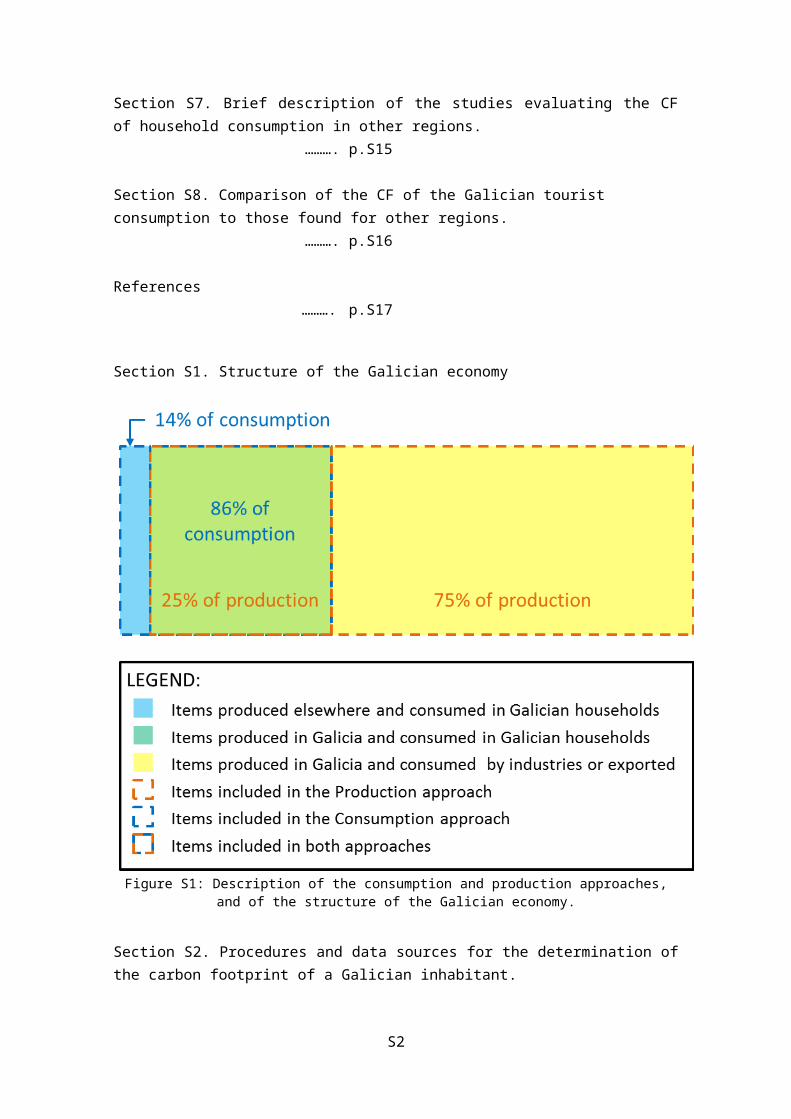
Section S1. Structure of the Galician economy

Figure S1: Description of the consumption and production approaches, and of the structure of the Galician economy.

Section S2. Procedures and data sources for the determination of the carbon footprint of a Galician inhabitant.

This section details the methodologies and data sources used to calculate the CF of a Galician inhabitant. The CF of the consumption of food, goods and services has been calculated using a top-down approach, while transport and housing were assessed through a bottom-up method (process analysis).

S2.1. Food, goods and transport

The CF of these categories has been calculated from the average yearly expenditures of a Galician inhabitant (INE, 2014c), expressed in euros and classified according to COICOP (Classification of Individual Consumption According to Purpose) categories. To determine the environmental impacts of the expenditures in each COICOP category, the US EIO database (Suh, 2010) has been used, which is implemented in SimaPro. Since the categories included in the COICOP classification do not match those included in the US EIO database, a transformation has been applied based on the tables provided by (Tukker et al., 2006), who adapted the US 480 commodity and service matrix to take into account European

S2

production characteristics as well as European substance emissions levels. Tukker transformation tables are based on the US IO database of 1998, while the 2002 database has been used here. The latter contains slightly different categories, and thus further transformations have been required in some of them: When a 2002 category corresponds to more than one 1998 category, the expenses of all 1998 categories have been aggregated in the corresponding 2002 item, while when several 2002 categories correspond to only one 1998 item, the expenses of the 1998 category have been equally divided among 2002 items. Galician consumption data refers to 2014, while US IO database is expressed in 2002 dollars. A monetary conversion has been done considering both currency conversion rates (FXTOP, 2016) and inflation (INE, 2016). To obtain the CF of all the consumption activities of the region, the following number of inhabitants has been assumed: 2,732,347 (IGE, 2015).

S2.2. Housing

The indispensable data required to calculate the CF of housing with process analysis is the total amount of inhabited dwellings of the region (divided between flats and houses), their average area and expected lifetime, to establish the share of the total emissions of the building process that correspond to each year of use. To determine the CF of utilities consumption, annual statistics of the amount of electricity, heat and water consumed per type of dwelling have been used. The annual amount of wastewater generated has also been estimated. Last, the yearly amount of waste generated per inhabitant and the waste management procedures applied were required, along with its transport characteristics. All data and data sources are summarized in table S1. All these values have been combined with life cycle inventories (LCI), taken from different sources (Table S1), to determine their associated CF.

S3

Table S1: Main statistical data used to determine the CF of housing. Data item Flat House LCI source Data sourceDwelling building

Number of dwellings 541,798 498,036 Cuéllar-Franca and Azapagic (2012) (IGE, 2010c) Average area (m2/dwelling) 90 121.5 Cuéllar-Franca and Azapagic (2012) (IGE, 2010b) Expected lifetime (y) 50 50 Cuéllar-Franca and Azapagic (2012) (CTE, 2009)

Electricity consumption (kWh/dwelling/y) 3250.12 3672.81 Ecoinvent: Electricity, low voltage | market for (Sech-Spahousec, 2011)Heat consumption (kWh/dwelling/y) 4055.71 11318.26

(Sech-Spahousec, 2011)

From coal 6.57 14.99 Ecoinvent: Heat, central or small-scale: heat, anthracite, at stove 5-15kW From liquefied petroleum gas 465.24 1169.30 Ecoinvent: Heat, central or small-scale: heat, light fuel oil, at boiler 10kW, non-mod. From diesel 832.61 2908.27 From natural gas 2743.98 1574.06 Ecoinvent: Heat, central or small-scale: heat, natural gas, at boiler mod <100kW Solar 7.30 284.83 Ecoinvent: Heat, central or small-scale: solar collector system, for hot water Geothermal 0.00 29.98 - From charcoal 0.00 59.96 Ecoinvent: Heat, central or small-scale: heat, charcoal, stove 5-15kW From firewood 0.00 5276.86 Ecoinvent: Heat, central or small-scale: heat, mixed logs, at wood heater 6kW

Water consumption (m3/inhabitant/y) 48.91 Ecoinvent: Tap water | market for (INE, 2012)

Wastewater treatment (m3/inhabitant/y) a 44.02b

Ecoinvent: Wastewater, average | treatment of, capacity 4.7E10l/year (49%)Ecoinvent: Wastewater, average | treatment of, capacity 1.1E10l/year (8%)Ecoinvent: Wastewater, average | treatment of, capacity 5E9l/year (31%)Ecoinvent: Wastewater, average | treatment of, capacity 1E9l/year (12%)Ecoinvent: Wastewater, average | treatment of, capacity 1.6E8l/year (1%)

(Hoekstra and Mekonnen, 2012)

Waste generation (kg/inhabitant/y) 383.92

(CMATI, 2014)

MSW sent to landfill 165.62 Ecoinvent: Municipal solid waste | treatment of, sanitary landfill MSW sent to incineration 154.37 Ecoinvent: Municipal solid waste | treatment of, incineration Organic sent to methanation 5.73 Ecoinvent: Methane, treatment of biogas, purification to methane Organic sent to composting 1.61 Ecoinvent: Bio waste| treatment of, composting Paper sent to recycling 8.17 Ecoinvent: Paper (waste treatment) | recycling of paper Glass sent to recycling 26.03 Ecoinvent: Packaging glass, white (waste treatment) | recycling Plastic sent to recycling 1.55 Ecoinvent: Mixed plastics (waste treatment) | recycling of mixed plastics Metal sent to recycling 2.04 Ecoinvent: Steel and iron (waste treatment) | recycling of steel and iron Other management options 18.79c -

Waste transport (kg fuel/t waste) 2.48 Ecoinvent: Waste collection service by 21 metric ton lorry (CMATI, 2011)a The amount of wastewater generated is assumed to be 90% of the tap water supplied.b Wastewater treatment plants have been split among sizes based on the actual size of the Galician plants, taken from (Augas de Galicia, 2016).c The amount of waste whose treatment is not specified has been proportionally assigned to the remaining categories.

S4

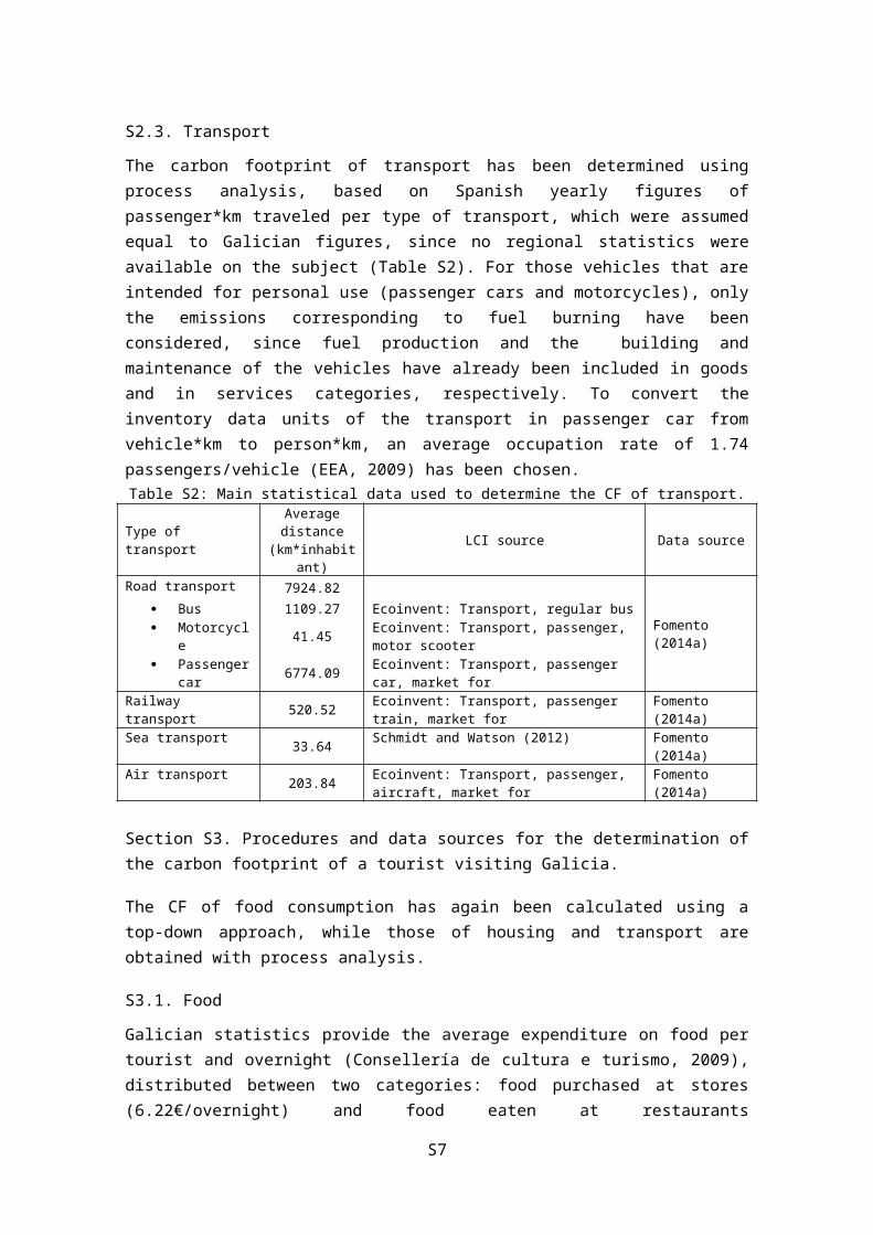
S2.3. Transport

The carbon footprint of transport has been determined using process analysis, based on Spanish yearly figures of passenger*km traveled per type of transport, which were assumed equal to Galician figures, since no regional statistics were available on the subject (Table S2). For those vehicles that are intended for personal use (passenger cars and motorcycles), only the emissions corresponding to fuel burning have been considered, since fuel production and the building and maintenance of the vehicles have already been included in goods and in services categories, respectively. To convert the inventory data units of the transport in passenger car from vehicle*km to person*km, an average occupation rate of 1.74 passengers/vehicle (EEA, 2009) has been chosen.

Table S2: Main statistical data used to determine the CF of transport.

Type of transportAverage distance

(km*inhabitant)LCI source Data source

Road transport 7924.82

Fomento (2014a) Bus 1109.27 Ecoinvent: Transport, regular bus Motorcycle 41.45 Ecoinvent: Transport, passenger, motor scooter Passenger car 6774.09 Ecoinvent: Transport, passenger car, market for

Railway transport 520.52 Ecoinvent: Transport, passenger train, market for Fomento (2014a)Sea transport 33.64 Schmidt and Watson (2012) Fomento (2014a)Air transport 203.84 Ecoinvent: Transport, passenger, aircraft, market

forFomento (2014a)

Section S3. Procedures and data sources for the determination of the carbon footprint of a tourist visiting Galicia.

The CF of food consumption has again been calculated using a top-down approach, while those of housing and transport are obtained with process analysis.

S3.1. Food

Galician statistics provide the average expenditure on food per tourist and overnight (Consellería de cultura e turismo, 2009), distributed between two categories: food purchased at stores (6.22€/overnight) and food eaten at restaurants (15.77€/overnight). Regarding the former, the same distribution among US EIO 2002 food categories that was considered for the Galician inhabitants has been assumed, while for the latter all expenditures have been assigned to one category: Food services and drinking places. Tourist consumption figures refer to 2009, so again a currency conversion was required to express them in US 2002 dollars. To obtain the yearly figure, the CF per overnight has been multiplied by the number of overnights spent in Galicia each year, obtained from different sources as detailed in the next section.

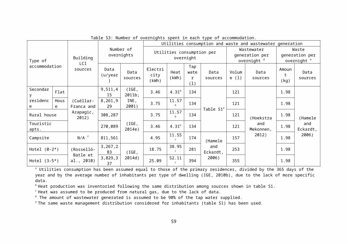
S3.2. Housing

To determine the CF of tourist accommodation, the same procedure as for the Galician inhabitants has been followed, based on the yearly number of overnights spent by the tourists in each type of facility, and on electricity, heat and water consumed, and on waste and wastewater generated, per tourist and overnight (Table S3). The same LCI data sources shown in Table S1 for housing have been used here.

S5

Table S3: Number of overnights spent in each type of accommodation.

Type of accommodation

Building LCI sources

Number of overnightsUtilities consumption and waste and wastewater generation

Utilities consumption per overnight Wastewater generation per overnight d

Waste generation per overnight e

Data (u/year)

Data sources

Electricity (kWh)

Heat (kWh)

Tap water

(l)

Data sources

Volume (l) Data sources Amount

(kg)Data

sources

Secondary residence

Flat(Cuéllar-Franca and Azapagic,

2012)

9,511,415 (IGE, 2011b;

INE, 2001)

3.46 4.31b 134

Table S1a

121

(Hoekstra and Mekonnen,

2012)

1.98

(Hamele and Eckardt,

2006)

House 8,261,929 3.75 11.57b 134 121 1.98

Rural house 308,287(IGE,

2014e)

3.75 11.57b 134 121 1.98Touristic apts. 270,089 3.46 4.31b 134 121 1.98Campsite N/A f 811,561 4.95 11.55c 174 (Hamele

and Eckardt, 2006)

157 1.98Hotel (0-2*) (Rosselló-Batle

et al., 2010)3,267,283 (IGE,

2014d)18.75 38.95c 281 253 1.98

Hotel (3-5*) 3,829,337 25.09 52.11c 394 355 1.98a Utilities consumption has been assumed equal to those of the primary residences, divided by the 365 days of the year and by the average number of inhabitants per type of dwelling (IGE, 2010b), due to the lack of more specific data.b Heat production was inventoried following the same distribution among sources shown in table S1.c Heat was assumed to be produced from natural gas, due to the lack of data.d The amount of wastewater generated is assumed to be 90% of the tap water supplied.e The same waste management distribution considered for inhabitants (table S1) has been used.f The emissions of the building of campsites were not accounted for due to the lack of inventory data. Nevertheless, the effects of this exclusion are expected to be of minor relevance.

S6

S3.3. Transport

Process analysis has been used to determine the emissions of tourist transport, based on the number of arrivals and on their countries of origin. The number of tourists coming to Galicia on a certain year is known (IGE, 2014c), divided into three categories according to their area of origin: Spain, Europe and Rest of the World. Tourists coming from Spain and Europe have been further stratified by region and country, respectively, based on a survey (Consellería de cultura e turismo, 2009). To determine the carbon footprint of these transport activities, the following assumptions have been made:

- Terrestrial transport has been assumed for those tourists coming from other regions of Spain or from Portugal. Terrestrial transport has been further stratified into five categories (Consellería de cultura e turismo, 2009): tourists coming by car (79.97%), bus (7.82%), train (6.19%), on foot or by bike (5.70%) and motorbike (0.33%). The high percentage of people arriving on foot or by bike responds to the pilgrimage to Santiago de Compostela.

- Intracontinental air transport has been assumed for those tourists coming from the rest of European countries.

- Intercontinental air transport has been assumed for those tourists coming from the Rest of the World.

- Average transport distances had to be determined from each region, and to do so the distance between the capital of each region/country to the capital of Galicia (Santiago de Compostela) has been determined. These distances have been doubled to consider the emissions of both the outbound and return journey, and have been taken from different sources for road (Google Maps, 2013) and air transport (TravelMath, 2016).

- To determine the transport distance of those tourists coming from the Rest of the World, Washington (United States of America) has been assumed as the city of origin, since more detailed statistics are not available, and the US is the non-European country from which more tourists come to Galicia (Turgalicia, 2016).

Table S4 summarizes the data used for each transport.

S7

Table S4: Number of arrivals per origin, distances covered and means of transport.Country/region of origin

Number of arrivals

Round trip distance (km)

Type of transport

LCI sources

Andalucía (Spain) 249,875 1,778

Terrestrial

Ecoinvent:-Transport, passenger car | market for

(80.0%)-Transport, passenger, motor scooter |

processing (0.3%)-Transport, regular bus | processing

(7.8%)-Transport, passenger train | market for

(6.2%)

Asturias (Spain) 159,559 608Castilla y León (Spain) 243,854 898

Cataluña (Spain) 286,002 2,208Madrid (Spain) 481,687 1,206Pais Vasco (Spain) 192,675 1,232C. Valenciana (Spain) 117,411 1,920

Rest of Spain 463,624 1,2001

Portugal 276,307 1,084France 102,536 2,190

Plane

Ecoinvent:- Transport, passenger, aircraft |

intracontinentalGermany 83,108 3,906United Kingdom 212,627 2,300Italy 110,091 3,462Switzerland 45,332 2,682

Rest of the world 249,32411,254

PlaneEcoinvent:

- Transport, passenger, aircraft | intercontinental)

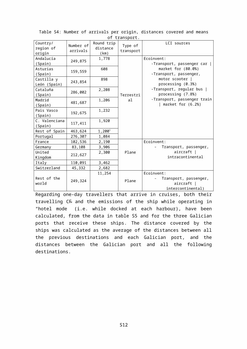
Regarding one-day travellers that arrive in cruises, both their travelling CF and the emissions of the ship while operating in “hotel mode” (i.e. while docked at each harbour), have been calculated, from the data in table S5 and for the three Galician ports that receive these ships. The distance covered by the ships was calculated as the average of the distances between all the previous destinations and each Galician port, and the distances between the Galician port and all the following destinations.

Table S5: Main data required to determine the CF of the tourists that arrive in cruises.

Data item PortA Coruña Ferrol Vigo

Number of passengers (u) 155701 (Autoridad

Portuaria de A Coruña, 2015)

10853 (Autoridad Portuaria de Ferrol-San Cibrao, 2015)

168808 (Autoridad Portuaria de Vigo,

2015)Average length of stay (h)

8.22 9.23 7.38

Average distance travelled (km)

855.35

(Autoridad Portuaria de A Coruña, 2015;

Searates, 2013)

797.42

(Autoridad Portuaria de Ferrol-San Cibrao, 2015; Searates, 2013)

882.73

(Autoridad Portuaria de Vigo,

2015; Searates, 2013)

LCI source (Simonsen, 2014)

Section S4. Procedures and data sources for the determination of the carbon footprint of Galician production.

This section describes the data sources used to determine the CF of each of the 8 subsectors considered in the production approach.

S4.1. Primary sector

Process analysis has been used to determine the CF of crop production, forestry, food of animal origin, fishing and aquaculture. Table S6 summarizes the data and data sources used to determine the CF of each category of the primary sector. It should be noted that, to determine

S8

the CF of crop production only the most abundant crops in the region have been inventoried, representing 96% in weight of the total production, and then a scaling factor has been used to evaluate the total impacts of crop growth in Galicia. Scaled values are shown in Table S6.

Table S6: Main data used to determine the CF of the production of the primary sector in Galicia.Category Product Amount Unit Data sources LCI sources

Crop production

Wheat grains 54,593,514 kg

(MAGRAMA, 2014a)

Ecoinvent: Wheat grain|wheat production

Rye grains 10,269,982 kg Ecoinvent: Rye grain |rye production

Maize grains 153,927,928 kg Ecoinvent: Maize grain |maize production

Beans 3,398,174 kg Ecoinvent: Fava bean |integrated production

Potatoes 495,720,012 kg Ecoinvent: Potato|production

Vineyard 130,894,155 kg (Villanueva-Rey et al., 2014)

Forage maize 2,608,577,253 kg (Roibás et al., 2016)Forage grass 4,537,188,584 kg

Cabbage 64,294,008 kg Ecoinvent: Cabbage white|production

Tomato 107,828,336 kg Ecoinvent: Tomato |production

Pepper 66,275,599 kg Ecoinvent: Green bell pepper|production

Green beans 44,319,456 kg Ecoinvent: : Fava bean |integrated production

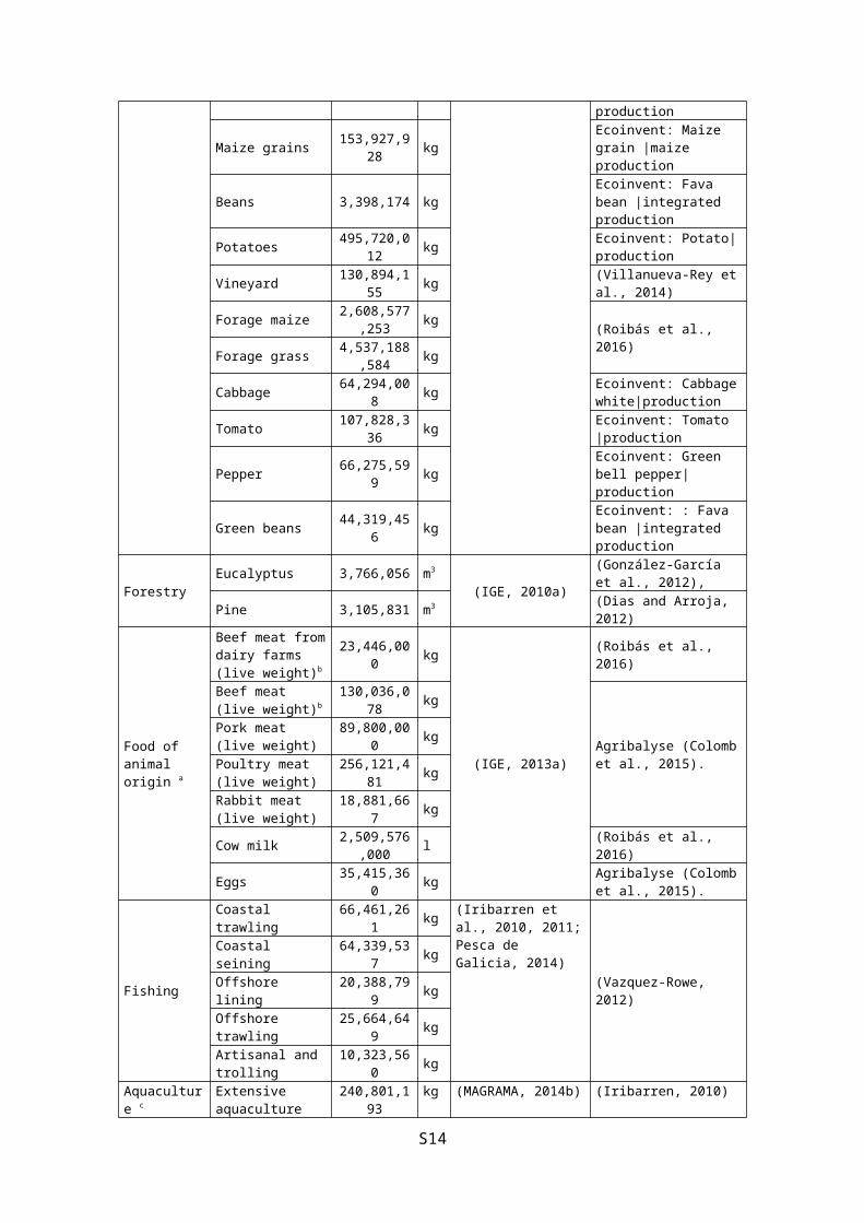
Forestry Eucalyptus 3,766,056 m3

(IGE, 2010a)(González-García et al., 2012),

Pine 3,105,831 m3 (Dias and Arroja, 2012)

Food of animal origin a

Beef meat from dairy farms (live weight)b

23,446,000 kg

(IGE, 2013a)

(Roibás et al., 2016)

Beef meat (live weight)b 130,036,078 kg

Agribalyse (Colomb et al., 2015).

Pork meat (live weight) 89,800,000 kg

Poultry meat (live weight) 256,121,481 kg

Rabbit meat (live weight) 18,881,667 kg

Cow milk 2,509,576,000 l (Roibás et al., 2016)

Eggs 35,415,360 kg Agribalyse (Colomb et al., 2015).

Fishing

Coastal trawling 66,461,261 kg (Iribarren et al., 2010, 2011; Pesca de Galicia, 2014) (Vazquez-Rowe, 2012)

Coastal seining 64,339,537 kgOffshore lining 20,388,799 kgOffshore trawling 25,664,649 kgArtisanal and trolling 10,323,560 kg

Aquaculture c

Extensive aquaculture 240,801,193 kg (MAGRAMA, 2014b)

(Iribarren, 2010)Intensive aquaculture 7,960,617 kg

a The following conversion figures have been used: dressing percentages (carcass weight/live weight) of beef (60%, (MAGRAMA, 2016)), pork (80%,Illescas et al. (2012)), poultry (67.5%, Peche (2009)) and rabbit (60%, MAGRAMA (1981)); and average egg weight: 60 g/egg (Colomb et al., 2015).b Beef meat production has been divided between meat produced as a by-product of the dairy farms and meat obtained at fattening farms based on (Roibás et al., 2016).c Mussel and turbot were used as a proxy for extensive and intensive aquaculture, respectively.

S9

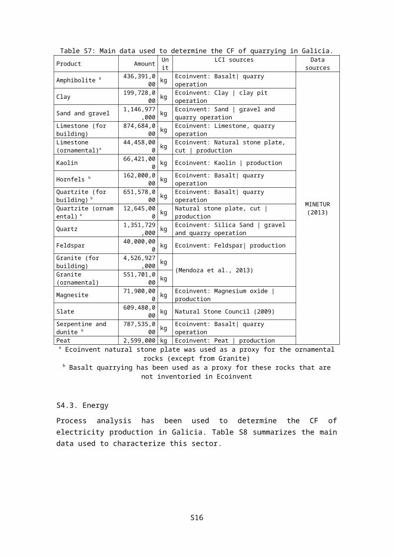
S4.2. Quarrying

Process analysis has been used to determine the CF of this category. Table S7 summarizes the main data used to characterize this sector.

Table S7: Main data used to determine the CF of quarrying in Galicia.Product Amount Unit LCI sources Data sourcesAmphibolite b 436,391,000 kg Ecoinvent: Basalt| quarry operation

MINETUR (2013)

Clay 199,728,000 kg Ecoinvent: Clay | clay pit operationSand and gravel 1,146,977,000 kg Ecoinvent: Sand | gravel and quarry operationLimestone (for building) 874,684,000 kg Ecoinvent: Limestone, quarry operationLimestone (ornamental)a

44,458,000 kg Ecoinvent: Natural stone plate, cut | production

Kaolin 66,421,000 kg Ecoinvent: Kaolin | productionHornfels b 162,000,000 kg Ecoinvent: Basalt| quarry operationQuartzite (for building) b 651,578,000 kg Ecoinvent: Basalt| quarry operationQuartzite (ornamental) a 12,645,000 kg Natural stone plate, cut | production

Quartz 1,351,729,000 kg Ecoinvent: Silica Sand | gravel and quarry operation

Feldspar 40,000,000 kg Ecoinvent: Feldspar| productionGranite (for building) 4,526,927,000 kg (Mendoza et al., 2013)Granite (ornamental) 551,701,000 kgMagnesite 71,900,000 kg Ecoinvent: Magnesium oxide | productionSlate 609,480,000 kg Natural Stone Council (2009)Serpentine and dunite b 787,535,000 kg Ecoinvent: Basalt| quarry operationPeat 2,599,000 kg Ecoinvent: Peat | production

a Ecoinvent natural stone plate was used as a proxy for the ornamental rocks (except from Granite)b Basalt quarrying has been used as a proxy for these rocks that are not inventoried in Ecoinvent

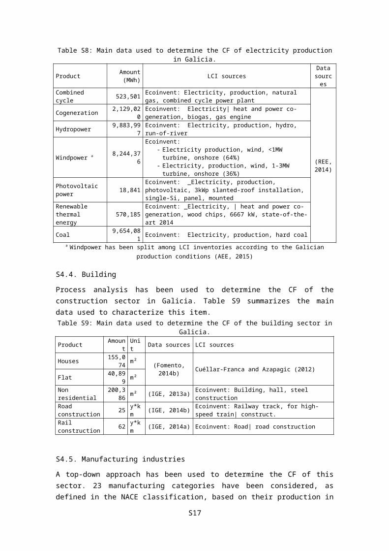
S4.3. Energy

Process analysis has been used to determine the CF of electricity production in Galicia. Table S8 summarizes the main data used to characterize this sector.

Table S8: Main data used to determine the CF of electricity production in Galicia.

Product Amount (MWh) LCI sources Data

sources

Combined cycle 523,501 Ecoinvent: Electricity, production, natural gas, combined cycle power plant

(REE, 2014)

Cogeneration 2,129,020 Ecoinvent: Electricity| heat and power co-generation, biogas, gas engine

Hydropower 9,883,997 Ecoinvent: Electricity, production, hydro, run-of-river

Windpower a 8,244,376Ecoinvent:

- Electricity production, wind, <1MW turbine, onshore (64%)- Electricity, production, wind, 1-3MW turbine, onshore (36%)

Photovoltaic power 18,841 Ecoinvent: _Electricity, production, photovoltaic, 3kWp slanted-roof installation, single-Si, panel, mounted

Renewable thermal energy 570,185 Ecoinvent: _Electricity, | heat and power co-generation, wood

chips, 6667 kW, state-of-the-art 2014Coal 9,654,081 Ecoinvent: Electricity, production, hard coal

a Windpower has been split among LCI inventories according to the Galician production conditions (AEE, 2015)

S4.4. Building

Process analysis has been used to determine the CF of the construction sector in Galicia. Table S9 summarizes the main data used to characterize this item.

S10

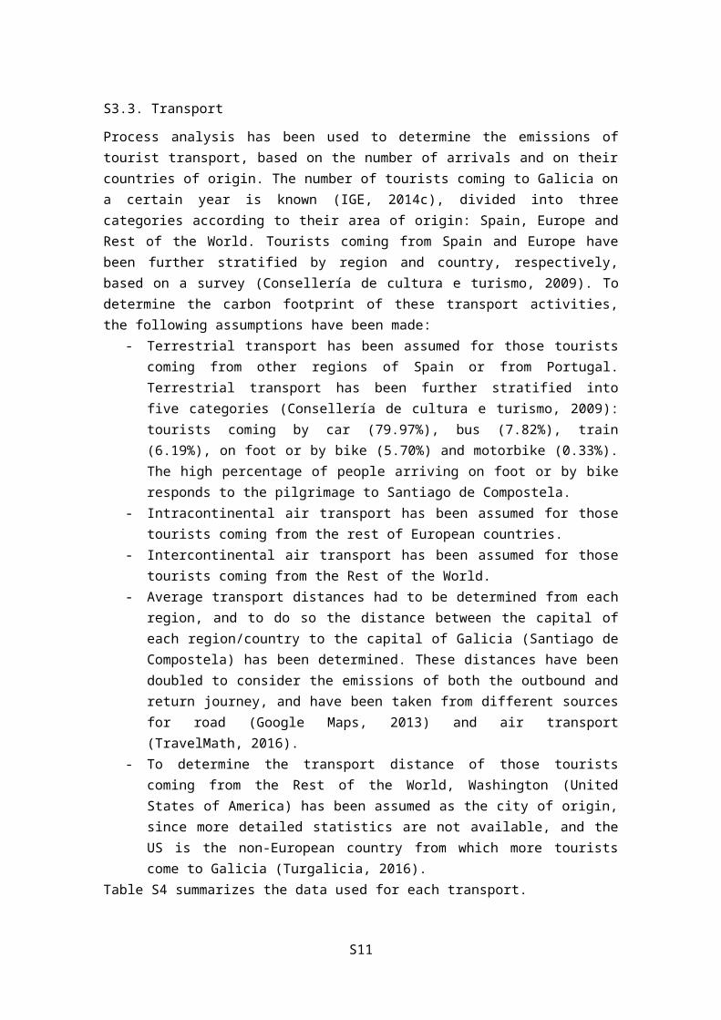
Table S9: Main data used to determine the CF of the building sector in Galicia.Product Amount Unit Data sources LCI sourcesHouses 155,074 m²

(Fomento, 2014b) Cuéllar-Franca and Azapagic (2012)Flat 40,899 m²Non residential 200,386 m² (IGE, 2013a) Ecoinvent: Building, hall, steel constructionRoad construction 25 y*km (IGE, 2014b) Ecoinvent: Railway track, for high-speed train| construct.Rail construction 62 y*km (IGE, 2014a) Ecoinvent: Road| road construction

S4.5. Manufacturing industries

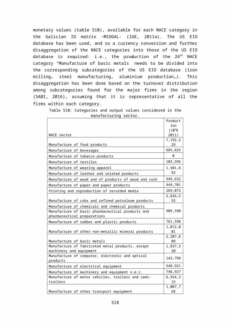
A top-down approach has been used to determine the CF of this sector. 23 manufacturing categories have been considered, as defined in the NACE classification, based on their production in monetary values (table S10), available for each NACE category in the Galician IO matrix –MIOGAL- (IGE, 2011a). The US EIO database has been used, and so a currency conversion and further disaggregation of the NACE categories into those of the US EIO database is required: i.e., the production of the 24 th NACE category “Manufacture of basic metals” needs to be divided into the corresponding subcategories of the US EIO database (iron milling, steel manufacturing, aluminium production…). This disaggregation has been done based on the turnover distribution among subcategories found for the major firms in the region (SABI, 2016), assuming that it is representative of all the firms within each category.

Table S10: Categories and output values considered in the manufacturing sector.

NACE sectorProduction(103€ 2011)

Manufacture of food products 7,192,229

Manufacture of beverages 685,825

Manufacture of tobacco products 0

Manufacture of textiles 103,396

Manufacture of wearing apparel1,501,892

Manufacture of leather and related products

Manufacture of wood and of products of wood and cork 949,632

Manufacture of paper and paper products 449,701

Printing and reproduction of recorded media 269,073

Manufacture of coke and refined petroleum products 2,826,555

Manufacture of chemicals and chemical products909,390

Manufacture of basic pharmaceutical products and pharmaceutical preparations

Manufacture of rubber and plastic products 761,598

Manufacture of other non-metallic mineral products 1,072,001

Manufacture of basic metals 2,207,809

Manufacture of fabricated metal products, except machinery and equipment 1,837,320

Manufacture of computer, electronic and optical products 143,798

Manufacture of electrical equipment 548,921

Manufacture of machinery and equipment n.e.c. 746,927

Manufacture of motor vehicles, trailers and semi-trailers 6,954,315

Manufacture of other transport equipment 1,007,768

Manufacture of furniture 472,425

Other manufacturing (e.g. jewellery, games, toys, …) 111,497

Repair and installation of machinery and equipment 1,114,315

S11

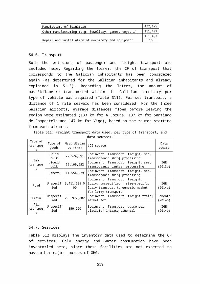
S4.6. Transport

Both the emissions of passenger and freight transport are included here. Regarding the former, the CF of transport that corresponds to the Galician inhabitants has been considered again (as determined for the Galician inhabitants and already explained in S1.3). Regarding the latter, the amount of mass*kilometre transported within the Galician territory per type of vehicle was required (Table S11). For sea transport, a distance of 1 mile seaward has been considered. For the three Galician airports, average distances flown before leaving the region were estimated (133 km for A Coruña; 137 km for Santiago de Compostela and 147 km for Vigo), based on the routes starting from each airport.

Table S11: Freight transport data used, per type of transport, and data sources.Type of

transportType of goods

Mass*distance (tkm) LCI source Data source

Sea transport

Solid bulk 22,524,391 Ecoinvent: Transport, freight, sea, transoceanic ship| processing

IGE (2013b)Liquid bulk 15,169,652 Ecoinvent: Transport, freight, sea, transoceanic tanker| processing

Others 11,554,229 Ecoinvent: Transport, freight, sea, transoceanic ship| processing

Road Unspecified 3,411,105,000Ecoinvent: Transport, freight, lorry, unspecified | size-specific lorry transport to generic market for lorry transport

IGE (2014a)

Train Unspecified 295,972,802 Ecoinvent: Transport, freight train| market for Fomento (2014b)

Air transport Unspecified 359,220 Ecoinvent: Transport, passenger, aircraft|

intracontinental IGE (2014b)

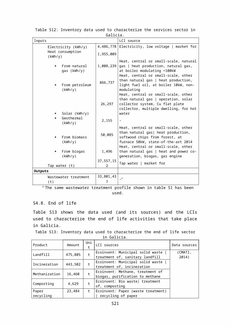
S4.7. Services

Table S12 displays the inventory data used to determine the CF of services. Only energy and water consumption have been inventoried here, since these facilities are not expected to have other major sources of GHG. Regarding energy consumption, only the amount of electricity consumed by the Galician service sector is available (MINETUR, 2012), while heat consumption is only available at the Spanish level (IDAE, 2013). Since electricity consumption is also available for the whole country, the rest of national figures have been extrapolated to Galicia based on the ratio between both electricity consumption figures. Tap water consumption in the service sector has been determined from the number of establishments of each type in Galicia (Cámara Santiago de Compostela, 2015). These establishments include stores, schools, restaurants, supermarkets… The full list of establishments considered, and the water consumption per type of establishment have been taken from section S.4.4 of Loiseau et al. (2014). A few examples of the type of establishemts are Water consumption figures used correspond to French statistics, which have been used due to the absence of regional (or Spanish) data. This assumption is not expected to have an important impact in the results, since the production of tap water used in the Galician services sector is not expected to be a major contributor to the total CF of the Galician production. Wastewater generation has been assumed to be a fixed percentage of the tap water supplied: 90% (Hoekstra and Mekonnen, 2012).

S12

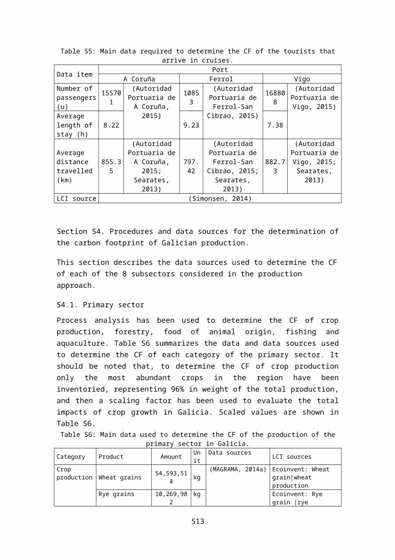
Table S12: Inventory data used to characterize the services sector in Galicia.Inputs LCI source

Electricity (kWh/y) 4,486,778 Electricity, low voltage | market for

Heat consumption (kWh/y) 1,955,009 From natural gas

(kWh/y) 1,008,239 Heat, central or small-scale, natural gas | heat production, natural gas, at boiler modulating <100kW

From petroleum (kWh/y)

866,737Heat, central or small-scale, other than natural gas | heat production, light fuel oil, at boiler 10kW, non-modulating

Solar (kWh/y)26,297

Heat, central or small-scale, other than natural gas | operation, solar collector system, Cu flat plate collector, multiple dwelling, for hot water

Geothermal (kWh/y) 2,155 -

From biomass (kWh/y)50,085

Heat, central or small-scale, other than natural gas| heat production, softwood chips from forest, at furnace 50kW, state-of-the-art 2014

From biogas (kWh/y) 1,496 Heat, central or small-scale, other than natural gas | heat and power co-generation, biogas, gas engine

Tap water (t) 37,557,152 Tap water | market for

Outputs

Wastewater treatment (t) 33,801,437 -a

a The same wastewater treatment profile shown in table S1 has been used.

S4.8. End of life

Table S13 shows the data used (and its sources) and the LCIs used to characterize the end of life activities that take place in Galicia.

Table S13: Inventory data used to characterize the end of life sector in Galicia.Product Amount Unit LCI sources Data sources

Landfill 475,805 t Ecoinvent: Municipal solid waste | treatment of, sanitary landfill

(CMATI, 2014)

Incineration 443,502 t Ecoinvent: Municipal solid waste | treatment of, incineration

Methanization 16,460 t Ecoinvent: Methane, treatment of biogas, purification to methane

Composting 4,629 t Ecoinvent: Bio waste| treatment of, composting

Paper recycling 23,484 t Ecoinvent: Paper (waste treatment) | recycling of paper

Glass recycling 74,789 t Ecoinvent: Packaging glass, white (waste treatment) | recycling

Plastic recycling 4,459 t Ecoinvent: Mixed plastics (waste treatment) | recycling of mixed plastics

Metal recycling 5,871 t Ecoinvent: Steel and iron (waste treatment) | recycling of steel and iron

Waste transport 2,597,372 kg fuel

Ecoinvent: Waste collection service by 21 metric ton lorry (CMATI, 2011)

Wastewater Treatment 375,486,158 m3 -a (Augas de Galicia,

2016)a The same wastewater treatment profile shown in table S1 has been used.

Section S5. Example of application of the double counting solving procedure

Table S14 represents a simplified version of the information contained in the Galician input-output matrix, in which only two productive sectors are shown (coke and refined petroleum; food products) and the flows with the remaining sectors and consumers are displayed in percentages instead of in monetary terms, for simplicity.

S13

When focusing on the “coke and refined petroleum sector”, the table displays which share of the total production (100%) is sold to another Galician sectors (intermediate consumption: 34%) or to the remaining users (66%). Since we consider that the CF of the share of the production which is used in another Galician sector (34%) has already been accounted for in the upstream processes of those sectors, we only consider the remaining 66% of the CF when summing up all the Galician sectors into the total productive activities.

Table S14: Simplified section of the Galician Input Output table.

Sector

Intermediate consumption (%) Remaining consumption (%) Total production

Primary sector

Services

Energy

Rest of sectors

TotalFinal consumption

Capital formation

Export Total

Coke and refined petroleum

4 2 7 21 34 13 1 51 66 100

Food products 10 6 0 9 25 18 1 56 75 100

The “coke and refined petroleum” sector has been chosen as the first example for simplicity, since energetic consumption is included in all the LCIs used to characterize the Galician sectors, and so only the share of “remaining consumption” is considered here when avoiding double counting. This was not the case for all sectors: the “food products” sector sells raw materials to the service sector (6%), but these are not accounted for in the upstream processes of the service sector, since only energetic inputs and water are included there. Similarly to the coke sector, when applying the procedure to the food products, only 75% of its CF is included there. The remaining 6% that should be accounted for in the services sector (but is not due to its limited inventory data) is removed from the food sector and added there, thus guaranteeing a proper consumer responsibility approach. So, the LCIs of each consuming sector have been analyzed individually to test which producing sectors were already accounted for, so as to adapt the aforementioned procedure to each case, and to obtain the corresponding multipliers.

Section S6. Individual results of the CF of the Galician productive activities

This section displays the individual results of the sectors considered in the production approach (table S15). The double-counting procedure has not been used here.

S14

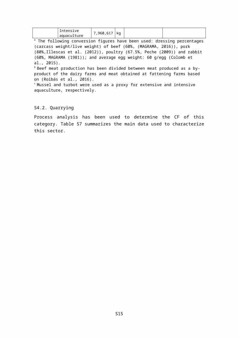
Table S15: Individual results of the CF of Galician productive activities. Sector Subsector CF (kt CO2e/y)

Primary sector

Crops 870

Forestry 244

Food of animal origin 5,425

Fishing and aquaculture 800

Quarrying 250

Energy 12,179

Building 159

Manufacture

Food products 8,660

Beverages 368

Textiles 70

Wearing apparel and leather 536

Wood and wood products 458

Paper and paper products 472

Printing 50

Coke and refined petroleum 3,919

Chemical and pharmaceutical 949

Rubber and plastic 583

Other non-metallic mineral 2,508

Basic metals 3,762

Fabricated metal products 1,377

Computer 30

Electrical 188

Machinery and equipment 293

Motor vehicles 3,183

Other transport 295

Furniture 194

Other manufacturing 34

Repair and installation 194

Transport 4,472

Services 36

End of life 499

Total 53,056

Section S7. Brief description of the studies evaluating the CF of household consumption in other regions.

Most of the studies included use Multi-Regional IO databases: Brizga et al. (2016) use the WIOD tables to determine the CF of consumption activities of households in Estonia, Latvia and Lithuania. Steen Olsen et al. (2016)‐ determined the CF of Norwegian household consumption by means of the Exiobase MRIO database. Shigetomi et al. (2014) used a simplified MRIO model adapted to the Japanese conditions, to determine the CF of the household consumption expenditures of different age groups in the country (a weighted average has been included here). Druckman and Jackson (2010) used a Quasi Multi Regional Input Output model to compare the current consumption patterns of UK households (which are included here) with a

S15

hypothetical, reduced consumption scenario. Other studies are based on Single Regional IO databases: Watson et al. (2013) used a SRIO approach to determine the CF of all European consumption activities in 2005 (households, 55% of the expenditures; government, 25%; and capital formation, 20%), which have been scaled here to represent household emissions only. Dey et al. (2007) determined the CF of the consumption activities of all the Australian states and the country average (which has been included here), using a SRIO methodology, adapted to some regional characteristics. And finally, only one study used a bottom-up approach to determine the CF of household consumption in Switzerland, by assimilating COICOP categories to certain LCA functional units (Girod and De Haan, 2010).

Section S8. Comparison of the CF of the Galician tourist consumption to those found for other regions.

Several studies have evaluated the carbon footprint of the touristic sector of particular countries or regions (Table S16).

Table S16: Comparison of the CF of the Galician tourism with those found for other countries. Region Approach Carbon footprint (g CO2e/€ GVA)

Switzerland Bottom-up 540

Wales Top-down 556

Austria Top-down 121

Sweden Top-down 687

UK Top-down 850

Spain Top-down 440

Galicia Hybrid 386

Perch-Nielsen et al. (2010) determined the CF of tourism in Switzerland following both a top-down and a bottom-up approach, and then applied their top-down methodology to other European countries (Austria, Spain, Sweden and the United Kingdom). Only the Swiss bottom-up results are included in table S16 since they are considered more reliable by their authors. Jones and Munday (2007) followed a top-down approach to calculate the CF of the touristic sector in Wales (United Kingdom). It should be noted that the system boundaries considered in these studies are different from those chosen here, as explained below, and so results should be compared with caution.Perch-Nielsen et al. (2010) consider the same system boundaries in their bottom-up (Switzerland) and top-down (Austria, Spain, Sweden and the United Kingdom) studies: only direct emissions coming from tourist companies resident in the studied country are considered (i.e. only the emissions of country-based firms, such as Swissair for Switzerland, are included). A similar top-down procedure is followed to determine the CF of the touristic sector in Wales (Jones and Munday, 2007). As the previous top-down studies, the CF is determined here based on economic data of the sector, and thus only the portion of the environmental impact that occurs as a result of increased economic demand in Wales is included (i.e. the portion of the visitors’ trip outside the region is not accounted for).Unlike the previous studies, the CF of tourist consumption is determined in our study following a hybrid approach. All the transport journeys of the tourists have been accounted for, from their places of origin to the final destination in Galicia, and they represent the larger source of impacts. However, some emissions have been excluded here (i.e. one-day trips and their

S16

associated transport emissions) due to the lack of data. Moreover, among the tourism activities, only food consumption has been considered, while the emissions coming from other leisure activities (i.e. sports, museums) were not accounted for. The aforementioned studies present their CF results per unit of Gross Value Added (GVA) attributable to tourism, a figure that can be found in the Tourism Satellite Account -TSA- (UNWTO, 2016) for numerous countries. Thus, our results have been expressed per unit of GVA and compared to those available for other European countries or regions (table 2). It should be noted that the Spanish TSA is only available for the whole country (INE, 2014b), and not for each of its regions, so the Galician Tourism GVA has been extrapolated from the Spanish one based on GDP data, which is available for the touristic sector both at the regional and national level (INE, 2014a). When expressed per unit of GVA, the results obtained are lower than those of the rest of the studies, with the exception of the Austrian ones, and similar to those obtained for Spain. Regarding the Austrian CF, their authors had already pointed out at an underestimation of the emissions caused by the inaccuracies found in the Austrian statistics. Only Swiss results are disaggregated into their major contributors: transport (87%), accommodation (10%) and food (2%). The remaining leisure activities only represent 1% of the emissions, demonstrating that their exclusion in our study should not affect the results in a significant way. The distribution among sectors is similar to the one found in our study, being transport the biggest contributor (59%), followed by accommodation (27%) and food (15%). The differences found can be explained both by the system boundaries used and the characteristics of the touristic sector in both regions.

References

AEE, 2015. Asociacion Empresarial Eólica. Mapa eólico de Galicia. http://www.aeeolica.org/es/map/galicia/ (accessed 10.10.2015).Augas de Galicia, 2016. EDAR de máis de 2000 h. eq. de Galicia. Depuradoras en funcionamento. http://augas.cmati.xunta.es/seccion-tema/c/Control_depuradoras_augas_residuais?content=/Portal-Web/Contidos_Augas_Galicia/Seccions/EDAR-2000-Galicia/seccion.html (accessed 04.04.2016).Autoridad Portuaria de A Coruña, 2015. Calendario de cruceros. http://www.puertocoruna.com/es/cruceros/cruceros/escalas.html (accessed 25.01.2016).Autoridad Portuaria de Ferrol-San Cibrao, 2015. Puerto ciudad: Cruceros. http://www.apfsc.com/castellano/puerto_ciudad/cruceros.html (accessed 25.01.2016).Autoridad Portuaria de Vigo, 2015. Cruceros: Previsión de Cruceros. http://www.apvigo.com/control.php?sph=a_lst_nrt=345%%a_lst_npa=6%%a_iap=1110 (accessed 25.01.2016).Brizga, J., Feng, K., Hubacek, K., 2016. Household carbon footprints in the Baltic States: A global multi-regional input–output analysis from 1995 to 2011. Appl. Energy http://dx.doi.org/10.1016/j.apenergy.2016.01.102 (in press).Cámara Santiago de Compostela, 2015. Fichero de empresas españolas. http://www.camaracompostela.com/index.asp?ind=1B0B0B0&p=110&tipo_listado=1 (accessed 04.05.2016).CMATI, 2011. Consellería de Medio Ambiente, Territorio e Infraestruturas. Xunta de Galicia. Plan de xestión de residuos urbanos de Galicia (PXRUG) 2010-2020.

S17

http://sirga.cmati.xunta.es/c/document_library/get_file?folderId=190428&name=DLFE-16055.pdf (accessed 04.04.2016).

CMATI, 2014. Consellería de Medio Ambiente, Territorio e Infraestruturas. Xunta de Galicia. Actualización do PXRUG 2010-2020. http://sirga.cmati.xunta.es/c/document_library/get_file?folderId=190428&name=DLFE-32998.pdf (accessed 04.04.2016).Colomb, V., Amar, S.A., Mens, C.B., Gac, A., Gaillard, G., Koch, P., Mousset, J., Salou, T., Tailleur, A., van der Werf, H.M., 2015. AGRIBALYSE®, the French LCI Database for agricultural products: high quality data for producers and environmental labelling, OCL, p. D104.Consellería de cultura e turismo, X.d.G., 2009. Enquisa de destino 2009. Análise estatística sobre o turismo en Galicia. http://www.turgalicia.es/aet/portal/docs/documentacion_vinculada/232.pdf (accessed 04.04.2016).CTE, 2009. Código Técnico de la Edificación. Documento básico: Seguridad Estructural. http://www.codigotecnico.org/images/stories/pdf/seguridadEstructural/DBSE.pdf (accessed 07.04.2016).Cuéllar-Franca, R.M., Azapagic, A., 2012. Environmental impacts of the UK residential sector: life cycle assessment of houses. Build. Environ. 54, 86-99.Dey, C., Berger, C., Foran, B., Foran, M., Joske, R., Lenzen, M., Wood, R., Birch, G., 2007. Household environmental pressure from consumption: an Australian environmental atlas, Water Wind Art and Debate. How environmental concerns impact on disciplinary research. Sydney University Press: Sydney, Australia, pp. 280-315.Dias, A.C., Arroja, L., 2012. Environmental impacts of eucalypt and maritime pine wood production in Portugal. J. Clean. Prod. 37, 368-376.Druckman, A., Jackson, T., 2010. The bare necessities: How much household carbon do we really need? Ecol. Econ. 69, 1794-1804.EEA, E.e.A., 2009. Car occupancy rates http://www.eea.europa.eu/data-and-maps/figures/term29-occupancy-rates-in-passenger-transport-1 (accessed 04/04/2016).Fomento, 2014a. Los transportes y las infraestructuras. Informe anual 2013. http://www.fomento.gob.es/MFOM.CP.Web/handlers/pdfhandler.ashx?idpub=BTW023 (accessed 04.04.2016).Fomento, 2014b. Observatorio del Ferrocarril en España. http://www.fomento.gob.es/Carreteras/Informe_Observatorio_Ferrocarril_2013.pdf (accessed 05.10.2015).FXTOP, 2016. Convertidor de divisas. http://fxtop.com/ (accessed 04.04.2016).Girod, B., De Haan, P., 2010. More or better? A model for changes in household greenhouse gas emissions due to higher income. J. Ind. Ecol. 14, 31-49.González-García, S., Moreira, M.T., Feijoo, G., Murphy, R.J., 2012. Comparative life cycle assessment of ethanol production from fast-growing wood crops (black locust, eucalyptus and poplar). Biomass Bioenergy 39, 378-388.Google Maps, 2013. https://www.google.es/maps/preview (accessed 11.11.2013).Hamele, H., Eckardt, S., 2006. Environmental initiatives by European tourism businesses. Instruments, indicators and practical examples. A contribution to the development of sustainable tourism in Europe, Ecotrans and University of Stuttgart, Life Environmental Programme of the European Commission.Hoekstra, A.Y., Mekonnen, M.M., 2012. The water footprint of humanity. Proc. Natl. Acad. Sci. USA 109, 3232-3237.IDAE, 2013. Instituto para la Diversificación y el Ahorro Energético. Detalle de consumos del Sector Servicios. http://www.idae.es/index.php/idpag.802/relcategoria.1368/relmenu.363/mod.pags/mem.detalle (accessed 05.10.2015).

S18

IGE, 2010a. Producción de madeira. http://www.ige.eu/igebdt/esqv.jsp?ruta=verTabla.jsp?OP=1&B=1&M=&COD=423&R=1[all];0[2010]&C=9912[12]&F=&S=&SCF= (accessed 10.10.2015).IGE, 2010b. Superficie media das vivendas segundo a clase de vivenda e tipo de edificio. http://www.ige.eu/igebdt/esqv.jsp?ruta=verTabla.jsp?OP=1&B=1&M=&COD=4354&R=1[all]&C=2[2010]&F=&S=0:0;998:12&SCF= (accessed 04.04.2016).IGE, 2010c. Vivendas segundo a clase de vivenda e tipo de edificio. Galicia. http://www.ige.eu/igebdt/esqv.jsp?ruta=verTabla.jsp?OP=1&B=1&M=&COD=4332&R=0[all]&C=1[1];2[2010]&F=&S=3:0&SCF= (accessed 07.04.2016).IGE, 2011a. Marco Input Output de Galicia 2011: Matriz simétrica da produción interior a prezos básicos. http://www.ige.eu/web/mostrar_actividade_estatistica.jsp?idioma=es&codigo=0307007003 (accessed 07.03.2016).IGE, 2011b. Vivendas por municipios segundo o tipo de vivenda. http://www.ige.eu/igebdt/esqv.jsp?ruta=verTabla.jsp?OP=1&B=1&M=&COD=5619&R=9915[12]&C=0[all]&F=&S=1:2011&SCF= (accessed 07.04.2016).IGE, 2013a. Principais producións gandeiras. http://www.ige.eu/igebdt/esqv.jsp?ruta=verTabla.jsp?OP=1&B=1&M=&COD=419&R=1[all];0[2013]&C=9912[12]&F=&S=&SCF= (accessed 10.10.2015).IGE, 2013b. Transporte marítimo de mercadorías nos portos de titularidade estatal. http://www.ige.eu/igebdt/esqv.jsp?ruta=verTabla.jsp?OP=1&B=1&M=&COD=442&R=1%5ball%5d&C=2%5b0%5d;0%5b2013%5d&F=&S=9916:108&SCF= (accessed 05.10.2015).IGE, 2014a. Toneladas quilómetro segundo comunidades autónomas de orixe e destino. Ano 2014. http://www.ige.eu/igebdt/esqv.jsp?ruta=verPpalesResultados.jsp?OP=1&B=1&M=&COD=6337&R=1[all]&C=2[all]&F=0:2014&S=&SCF= (accessed 07.03.2016).IGE, 2014b. Tráfico de transporte nos aeroportos. http://www.ige.eu/igebdt/esqv.jsp?ruta=verTabla.jsp?OP=1&B=1&M=&COD=443&R=2[all];0[2014]&C=1[2];3[0]&F=&S=9916:108&SCF= (accessed 05.10.2015).IGE, 2014c. Viaxeiros entrados e noites en establecementos hoteleiros e de turismo rural por procedencia. http://www.ige.eu/igebdt/esqv.jsp?ruta=verTabla.jsp?OP=1&B=1&M=&COD=1945&R=9928[12];2[all];0[2014]&C=1[all];3[all]&F=&S=&SCF= (accessed 05.04.2016).IGE, 2014d. Viaxeiros entrados e noites en establecementos hoteleiros por categoría. http://www.ige.eu/igebdt/esqv.jsp?ruta=verTabla.jsp?OP=1&B=1&M=&COD=1947&R=9928[12];0[2014];1[all]&C=2[all]&F=&S=&SCF= (accessed 04.04.2016).IGE, 2014e. Viaxeiros, noites e estadía media por país de residencia e tipo de aloxamento. http://www.ige.eu/igebdt/esqv.jsp?ruta=verTabla.jsp?OP=1&B=1&M=&COD=4785&R=9928[12];1[all];0[2014]&C=2[all];3[0]&F=&S=&SCF= (accessed 04.04.2016).IGE, 2015. Poboación segundo sexo e idade. http://www.ige.eu/igebdt/esqv.jsp?ruta=verTabla.jsp?OP=1&B=1&M=&COD=590&R=9912[12];2[2013:2014:2015];0[0]&C=1[0]&F=&S=&SCF= (accessed 05.04.2016).Illescas, J.L., Ferrer, S., Bacho, O., 2012. Porcino. Guía práctica. http://www.mercasa.es/files/multimedios/1368093648_guiaporcino.pdf (accessed 12/04/2016).INE, 2001. Censos de Población y Viviendas 2001. Resultados definitivos. http://www.ine.es/censo/es/inicio.jsp (accessed 04.04.2016).

S19

INE, 2012. Encuesta sobre el suministro y saneamiento de agua. http://www.ine.es/prensa/np872.pdf (accessed 04.04.2016).INE, 2014a. Contabilidad Regional de España. Base 2010. Serie contable. http://www.ine.es/daco/daco42/cre00/b2010/dacocre_base2010.htm (accessed 25.05.2016).INE, 2014b. Cuenta satélite del turismo de España. Base 2010. Serie contable 2010-2014. http://www.ine.es/dynt3/inebase/index.htm?type=pcaxis&path=/t35/p011/base_2010/serie/&file=pcaxis (accessed 28.06.2016).INE, 2014c. Gasto total y gastos medios de los hogares. http://www.ine.es/jaxiT3/Datos.htm?t=10724 (accessed 03.03.2016).INE, 2016. Cálculo de variaciones del Indice de Precios de Consumo (sistema IPC base 2011). http://www.ine.es/varipc/ (accessed 05.04.2016).Iribarren, D., 2010. Life Cycle Assessment of mussel and turbot aquaculture. Application and insights, Group of Environmental Engineering and Bioprocesses. University of Santiago de Compostela.Iribarren, D., Vázquez-Rowe, I., Hospido, A., Moreira, M.T., Feijoo, G., 2010. Estimation of the carbon footprint of the Galician fishing activity (NW Spain). Sci. Total Environ. 408, 5284-5294.Iribarren, D., Vázquez-Rowe, I., Hospido, A., Moreira, M.T., Feijoo, G., 2011. Updating the carbon footprint of the Galician fishing activity (NW Spain). Sci. Total Environ. 409, 1609-1611.Jones, C., Munday, M., 2007. Exploring the environmental consequences of tourism: a satellite account approach. J. Travel Res. 46, 164–172.Loiseau, E., Roux, P., Junqua, G., Maurel, P., Bellon-Maurel, V., 2014. Implementation of an adapted LCA framework to environmental assessment of a territory: important learning points from a French Mediterranean case study. J. Clean. Prod. 80, 17-29.MAGRAMA, 1981. Caracterizacion de la canal y calidad de la carne del conejo consumido en España. Boletín de Cunicultura Nº 16 29-32.MAGRAMA, 2014a. Anuario de estadística 2013. http://www.magrama.gob.es/es/estadistica/temas/publicaciones/anuario-de-estadistica/2013/default.aspx (accessed 10.10.2015).MAGRAMA, 2014b. Datos de producción de acuicultura. http://www.magrama.gob.es/app/jacumar/datos_produccion/lista_datos_produccion.aspx?Id=es (accessed 10.10.2015).MAGRAMA, 2016. Raza bovina RUBIA GALLEGA. http://www.magrama.gob.es/es/ganaderia/temas/zootecnia/razas-ganaderas/razas/catalogo/autoctona-fomento/bovino/rubia-gallega/usos_sistema.aspx (accessed 12.04.2016).Mendoza, J.-M.F., Feced, M., Feijoo, G., Josa, A., Gabarrell, X., Rieradevall, J., 2013. Life cycle inventory analysis of granite production from cradle to gate. Int. J. Life Cycle Assess. 19, 153-165.MINETUR, 2012. Consumos energía electrica en Galicia 2012. http://www.minetur.gob.es/energia/balances/Publicaciones/ElectricasAnuales/Paginas/ElectricasAnuales.aspx (accessed 05.10.2015).MINETUR, 2013. Minerva. Estadísticas de producción minera. https://sedeaplicaciones.minetur.gob.es/Minerva/GenerarInformes.aspx (accessed 07.03.2016).Natural Stone Council, 2009. Slate Quarrying and Processing: A Life-Cycle Inventory http://www.naturalstonecouncil.org/content/file/LCI%20Reports/LCI_Slate_LCIv1_Sept2009.pdf (accessed 19.04.2016).Peche, G.A., 2009. Costo de producción del pollo. Selecciones avícolas.Perch-Nielsen, S., Sesartic, A., Stucki, M., 2010. The greenhouse gas intensity of the tourism sector: The case of Switzerland. Environ. Sci. Policy 13, 131-140.Pesca de Galicia, 2014. Estatísticas: Vendas nas Lonxas (Agrupado por Especie). http://www.pescadegalicia.com/estadisticas.html (accessed 10.10.2015).

S20

REE, 2014. El sistema eléctrico español. http://www.ree.es/es/publicaciones/sistema-electrico-espanol/informe-anual/informe-del-sistema-electrico-espanol-2014 (accessed 07.03.2016).Roibás, L., Martínez, I., Goris, A., Barreiro, R., Hospido, A., 2016. An analysis on how switching to a more balanced and naturally improved milk would affect consumer health and the environment. Sci. Total Environ. 566–567, 685-697.Rosselló-Batle, B., Moià, A., Cladera, A., Martínez, V., 2010. Energy use, CO2 emissions and waste throughout the life cycle of a sample of hotels in the Balearic Islands. Energy Build. 42, 547-558.SABI, 2016. Sistema de Análisis de Balances Ibéricos. Bureau Van Dijk. http://www.buc.unican.es/content/sabisistemaanalisisbalancesibericos (accessed 05.10.2016).Schmidt, J., Watson, J., 2012. Eco Island Ferry–comparative LCA of island ferry with carbon fibre composite based and steel based structures. 2-0 LCA consultants. Aalborg, Denmark.Searates, 2013. http://www.searates.com/reference/portdistance/ (accessed 11.11.2013).Sech-Spahousec, P., 2011. Análisis del consumo energético del sector residencial en España. http://www.idae.es/uploads/documentos/documentos_Informe_SPAHOUSEC_ACC_f68291a3.pdf (accessed 04.04.2016).Shigetomi, Y., Nansai, K., Kagawa, S., Tohno, S., 2014. Changes in the carbon footprint of Japanese households in an aging society. Environ. Sci. Technol. 48, 6069-6080.Simonsen, M., 2014. Cruise ship tourism - a LCA analysis. http://transport.vestforsk.no/Dokumentasjon/pdf/Skip/Cruise.pdf (accessed 08.03.2016).Steen Olsen, K., Wood, R., Hertwich, E.G., 2016. The carbon footprint of Norwegian household ‐consumption 1999–2012. J. Ind. Ecol. 20, 582–592.Suh, S., 2010. CEDA 4.0 User’s Guide. https://www.pre-sustainability.com/download/manuals/CEDAUsersGuide.pdf (accessed 03/03/2016).TravelMath, 2016. Flight calculator. http://www.travelmath.com/flights/ (accessed 05.04.2016).Tukker, A., Huppes, G., Guinée, J.B., Heijungs, R., de Koning, A., van Oers, L., Suh, S., Geerken, T., van Holderbeke, M., Jansen, B., Nielsen, P., 2006. Environmental Impact of Products (EIPRO) Analysis of the life cycle environmental impacts related to the final consumption of the EU-25. European Commission, Joint research Centre (DG JRC). Institute for Prospective Technological Studies, pp. 1 - 136.Turgalicia, 2016. Conxuntura hoteleira en Galicia http://www.turgalicia.es/aet/portal/index.php?idm=16 (accessed 07.04.2016).UNWTO, 2016. The conceptual framework for TSA - Tourism Satellite Account: Recommended Methodological Framework http://statistics.unwto.org/content/tsarmf2008 (accessed 28.06.2016).Vazquez-Rowe, I., 2012. Fishing for solutions: Environmental and operational assessment of selected Galician fisheries and their products, Group of Environmental Engineering and Bioprocesses. University of Santiago de Compostela.Villanueva-Rey, P., Vázquez-Rowe, I., Moreira, M.T., Feijoo, G., 2014. Comparative life cycle assessment in the wine sector: biodynamic vs. conventional viticulture activities in NW Spain. J. Clean. Prod. 65, 330-341.Watson, D., Acosta Fernandez, J., Wittmer, D., Pedersen, O.G., 2013. Environmental pressures from European consumption and production: a study in integrated environmental and economic analysis. http://www.eea.europa.eu/publications/environmental-pressures-from-european-consumption/at_download/file (accessed 25.10.2016).

S21