Universitat Rovira i Virgili Escola Tècnica Superior d’Enginyeria

MASTER THESIS

A multicriteria decision aid approach for the management of biosolids generated at

wastewater treatment plants

Josep Pijuan Parra <josep.pijuan@estudiants.urv.cat>

Director: Dr. Aïda Valls Mateu

Tarragona, 2009

 

iv

Agraïments

La realització d’aquesta tesis ha estat possible gràcies al suport del projecte (CTM2007-64490/TECNO), finançat pel Ministerio de Medio Ambiente i al suport del projecte CENIT SOSTAQUA.

En primer lloc, m’agradaria donar les gràcies més sinceres a la meva directora, Aïda Valls, per tot el suport, dedicació i consells rebuts, així com per la confiança que ha dipositat en mi. En segon lloc, vull agrair a la Dra. Marta Schuhmacher la oportunitat que m’ha donat d’iniciar-me en la recerca i de poder treballar en un projecte d’investigació d’aquestes característiques. També apreciar els comentaris i suggeriments rebuts de Jordi Sierra, Roman Słowiński i Jozo Dujmović, que han permès aprofundir aquesta tesis.

Vull dedicar aquestes línies als meus companys del grup ITAKA amb els que he compartit bones estones i a totes les persones que formen part de l’equip d’investigació del Projecte. Vull fer especial menció a Ana Passuello, la qual m’ha ajudat en tot moment i a qui li desitjo tota la sort del món ara i sempre.

No em puc oblidar de donar les gràcies a totes les persones que d’una manera o d’una altra han cregut en mi i m’han fet costat durant aquests últims dos anys, gràcies a tots. I finalment, el més sentit agraïment als meus pares pel seu suport incondicional durant tota la meva vida, al meu germà per la seva ajuda i a la meva novia per la seva gran paciència; a tots ells va dedicada aquesta tesis.

v

 

vi

 Contents

1.  Introduction ..................................................................................................... 1 1.1.  Biosolid management ............................................................................. 2 1.2.  Aims of the Master Thesis ...................................................................... 3 1.3.  Document structure................................................................................. 4 

2.  State of the art: MCDA methods and tools...................................................... 5 2.1.  MCDA definitions .................................................................................. 5 2.2.  Preference modeling ............................................................................... 7 2.3.  Nature of information ............................................................................. 8 2.4.  Dominance and efficiency ...................................................................... 9 2.5.  MAUT methods .................................................................................... 12 2.6.  Outranking methods.............................................................................. 14 2.7.  Multi-objective methods ....................................................................... 16 2.8.  Rule-based methods.............................................................................. 17 2.9.  Decision process ................................................................................... 19 2.10.  Decision problem formulation .............................................................. 21 2.11.  MCDM in environment ........................................................................ 22 2.12.  Decision Tools ...................................................................................... 23 

3.  Our proposal: a decision support system for sewage sludge application in agricultural soils ......................................................................................................... 27 

3.1.  Define the problem ............................................................................... 27 3.2.  Determine requirements........................................................................ 28 3.3.  Establish goals ...................................................................................... 28 3.4.  Identify alternatives and define criteria ................................................ 29 

3.4.1.  Introduction to criteria hierarchy...................................................... 30 3.4.2.  First approach: Soil & landscape...................................................... 31 3.4.3.  Second approach: Soil, landscape & sludge ..................................... 33 3.4.4.  Architecture of the MCDA system................................................... 34 3.4.5.  Input data.......................................................................................... 35 3.4.6.  Building utility functions.................................................................. 39 

3.5.  Fuzzy Expert Systems........................................................................... 44 3.6.  Modeling utilities with fuzzy expert systems........................................ 46 

3.6.1.  Defined Expert Systems ................................................................... 47 3.6.2.  An example: the Organic Matter criterion........................................ 51 

3.7.  Select a decision making tool ............................................................... 56 3.8.  Logic Scoring of Preference (LSP)....................................................... 57 3.9.  Aggregation of utilities with LSP ......................................................... 62 3.10.  Flow of execution ................................................................................. 68 

vii

4.  Used Data and results .................................................................................... 69 4.1  Data....................................................................................................... 69 4.2  Evaluate alternatives against criteria..................................................... 71 4.3  Rating and evaluation of results............................................................ 76 4.4  Validation ............................................................................................. 86 4.5  Sensitivity Analysis .............................................................................. 87 

4.5.1.  Sensitivity with respect to the weights ............................................. 88 4.5.2.  Results of the weights sensitivity analysis........................................ 89 

5.  Conclusions and future work ....................................................................... 102 6.  Bibliography................................................................................................ 105 

viii

List of Figures

Figure 2.1 An example of two alternatives.............................................................. 9 Figure 2.2 An example where a utopian alternative does not exist. ...................... 10 Figure 2.3 Pairs of alternatives in Pareto dominance relationships. Case I ........... 11 Figure 2.4 Pairs of alternatives in Pareto dominance relationships. Case II.......... 11 Figure 2.5 Pairs of alternatives in Pareto dominance relationships. Case III ........ 12 Figure 2.6 Thresholds in a criterion ...................................................................... 15 Figure 3.1 Hierarchy of criteria ............................................................................. 34 Figure 3.2: Decision support system architecture ................................................. 35 Figure 3.3 Utility functions for environmental and human health simple criteria. 40 Figure 3.4 Structure of a Fuzzy Expert System..................................................... 45 Figure 3.5 Fuzzy linguistic terms for the Utility ................................................... 46 Figure 3.6 Groundwater vulnerability ................................................................... 47 Figure 3.7 Groundwater contamination expert system.......................................... 48 Figure 3.8 Human health risk, ingestion dose expert system ................................ 48 Figure 3.9 Human health risk, labor expert system............................................... 49 Figure 3.10 Soil biodiversity expert system .......................................................... 49 Figure 3.11 Soil nitrates expert system ................................................................. 49 Figure 3.12 Soil pH expert system ........................................................................ 50 Figure 3.13 Soil contamination expert system ...................................................... 50 Figure 3.14 Soil organic matter expert system...................................................... 51 Figure 3.15 Input linguistic variables for the Organic Matter complex criterion .. 52 Figure 3.16 Output linguistic variables for the Organic Matter complex criterion53 Figure 3.17 The rule blocks in fuzzyTECH ........................................................... 54 Figure 3.18 Example1: Compost sludge with much organic matter and a soil

without organic matter ................................................................................................ 55 Figure 3.19 Example2: Sludge with an uncertain OM level ................................. 56 Figure 3.20 Simultaneity/replaceability related to addness and orness ................. 59 Figure 3.21 Analytica nodes: Variable, Function.................................................. 62 Figure 3.22 MCDA Tool model representation....................................................... 1 Figure 3.23 A simple utility function on Analytica............................................... 65 Figure 3.24 Mathematical functions implemented on Analytica........................... 66 Figure 3.25 Decision Making model for biosolid management with Analytica.... 67 Figure 3.26 Decision Support System execution flow .......................................... 68 Figure 4.1 Example of pH expert system evaluating alternative 1........................ 74 Figure 4.2 MCDA Tool model representation......................................................... 1 Figure 4.3 Results of soil1 aggregation node ........................................................ 78 Figure 4.4 Results of soil2 aggregation node ........................................................ 78 

ix

Figure 4.5 Results of groundwater aggregation node............................................ 79 Figure 4.6 Results of population aggregation node............................................... 80 Figure 4.7 Results of landscape aggregation node ................................................ 80 Figure 4.8 Results of soil aggregation node .......................................................... 81 Figure 4.9 Results of population risk aggregation node ........................................ 82 Figure 4.10 Results of exposure risk aggregation node......................................... 83 Figure 4.11 Results of economical aggregation node............................................ 83 Figure 4.12 Results of environmental risk aggregation node ................................ 84 Figure 4.13 Results of human health risk aggregation node.................................. 85 Figure 4.14 Results of general evaluation aggregation node................................. 85 Figure 4.15 Levels in the sensitivity analysis........................................................ 88 Figure 4.16 Scheme of the calculation for Level I: General evaluation ................ 89 Figure 4.17 Results of general evaluation sensitivity analysis .............................. 90 Figure 4.18 Results of human health risk evaluation sensitivity analysis ............. 91 Figure 4.19 Results of economic sensitivity analysis............................................ 92 Figure 4.20 Results of environmental sensitivity analysis .................................... 93 Figure 4.21 Results of exposure risk sensitivity analysis ...................................... 94 Figure 4.22 Results of soil sensitivity analysis...................................................... 95 Figure 4.23 Results of groundwater sensitivity analysis ....................................... 96 Figure 4.24 Results of population risk sensitivity analysis ................................... 97 Figure 4.25 Results of soil1 sensitivity analysis.................................................... 98 Figure 4.26 Results of soil2 sensitivity analysis.................................................... 99 Figure 4.27 Results of population sensitivity analysis ........................................ 100 Figure 4.28 Results of landscape sensitivity analysis.......................................... 101 

x

List of Tables

Table 2.1 Decision matrix ..................................................................................... 13 Table 2.2 List of the most popular Decision Tools................................................ 26 Table 3.1 Outline of the criteria structure.............................................................. 32 Table 3.2 Sludge input data, sludge criteria and sludge criteria abbreviations...... 36 Table 3.3 Soil and landscape input data ................................................................ 38 Table 3.4 Other input data ..................................................................................... 38 Table 3.5 Complex criteria dependences............................................................... 43 Table 3.6 Utility values for the different combinations of values related to the

organic matter criterion............................................................................................... 53 Table 3.7 Logic Scoring Preference operators based in CPL ................................ 61 Table 4.1 Table of the WWTP types used to take sludge samples for the test phase

.................................................................................................................................... 70 Table 4.2 Landscapes types used to take the soil samples in the test phase .......... 70 Table 4.3 Set of alternatives in the case study....................................................... 70 Table 4.4 Criteria abbreviations ............................................................................ 71 Table 4.5 Data for each input property.................................................................. 72 Table 4.6 Utility values from Expert systems........................................................ 73 Table 4.7 Utility values from simple criteria......................................................... 75 Table 4.8 Ranking of soils with respect to WWTP sewage sludge ...................... 86 Table 4.9 Initial weights and proposed weights for criteria of soil1 node............. 98 

1

1. Introduction

The research conducted in this Master Thesis is part of the Spanish project (CTM2007-64490/TECNO): “Desarrollo de un modelo de evaluación de exposición y riesgo por la aplicación de fangos de depuradoras en suelo agrícola, basado en un sistema experto integrado en SIG”, funded by the “Programa Nacional de Ciencias y Tecnologías Medioambientales” of the Environmental Ministry. The project is 3 years long, it started at 2008 and it is going to finish at the end of 2010.

In this research project, a multi-disciplinary team studies all the factors to take into account in the decision process of selecting the best use of sewage sludge produced at waste water treatment plants. The following groups are involved in this project.

- Anàlisi i Gestió Ambiental (AGA), Department of Chemist Engineering

on ETSEQ, URV. - Laboratorio de Toxicología y Salud Medioambiental, Department of

Medical Sciences, FMCS, URV. - Laboratorio de edafología, Faculty of Pharmacy, Universitat de

Barcelona (UB). - Análisis Territorial i Estudios Turísticos (GRATET), Pre-departmental

unit of Geography, FLL, URV. - Intelligent Technologies for Advanced Knowledge Acquisition (ITAKA),

Department of Computer Science and Mathematics, ETSE, URV. This funded research project is separated in some stages. The following are the

main objectives of this project:

1. A laboratory study of the major processes governing the mobility, bioavailability and toxicity of contaminants (heavy metals and organic compounds). In this stage different analysis on soils and sludge are done.

2. Field-level study to determine the soil-vegetation-transfer leaching and toxicity.

3. Development and validation of models of transmission and distribution. This stage is composed by the elaboration of a tridimensional (Neuro-fuzzy) model of flow and transport through the subsoil and groundwater pollutants in diffuse by the application of sludge in agricultural soils.

4. Modeling of exposure and risk for population and ecosystems 5. Development of vulnerability indices based on soil characteristics, type

of sludge and crop type. Development of a vulnerability index that includes the characteristics of soil, sludge and vegetation.

2

6. Prepare a guide of recommendations In this Master Thesis we have been working on the design and implementation of a

tool for supporting the points three and five, where fuzzy methods and a vulnerability index (utility) are required. Finally the decision tool will be used to build a set of recommendations for the usage of biosolids in agricultural soils.

The management of sewage sludge generated in wastewater treatment plants is a complex problem. This problem has a lot of associated costs at an economical level, but also important impacts to humans and ecosystems.

Before presenting the goals of this Master Thesis in detail, a brief explanation of the environmental problem of sewage sludge management is given.

1.1. Biosolid management

Biosolids, also referred as sewage sludge, are residues generated at wastewater treatment plants (WWTP), obtained from solids removal on various parts of the treatment system. In Spain the generation of biosolids increased in a 39% from 1997 to 2005[PNLD, 2008]. Since the application of the legislation [RDL 11/1995)] which requires building new plants in towns with a population higher than 2000 inhabitants, more than 1000 WWTP have been build in all Spanish region.

Once treated, the amount of sludge can be recycled or disposed using three main routes: disposal on agricultural soil, incineration and landfill. Any of these three scenarios leads to different impacts to humans and ecosystem.

The sewage sludge application on soil improves fertility and exempt fertilizers use. Furthermore the nitrates content of soil increases crop production. For these reasons, the Spanish government wants that at least 70% of the WWTP sludge is applied into agricultural soils. In 2005 the recycling of sewage sludge to agriculture represented a 65% of the total disposal of biosolids [PNLD, 2008], but it should be studied how this percentage may be increased. Even so, biosolid application on soils may lead to groundwater nitrification as a result of nitrogen movement through lixiviate. The nitrates content of biosolids is a variable related to application dose. Some studies have proven that biosolids application improves soil fertility along the years [Fuentes et al., 2007]. However, care must be taken on areas that are vulnerable to nitrogen pollution, as recommended on EC Nitrate Directive 91/676.

The application of sewage sludge as a combustible is another possibility to take into account for the rest of the sewage sludge not used in agricultural soils. This option is especially interesting for cement plants because they can use instead of other fuel types. In order to be incinerated, sewage sludge must have a drying treatment, which increases the costs.

Finally the last and less preferred destination for sewage sludge is to be disposed in a landfill. Usually it happens when the level of metal contaminants present in the sludge exceed the maximum level required by the Spanish legislation for the application on agricultural soils, or even to incineration.

However, legislation is not concerned on any other kind of impacts to humans and ecosystem, such as the exposition to organic contaminants through different routes

3

(inhalation, ingestion and dermal contact), the lifecycle, and the field properties. For this reason, in the Spanish project mentioned before, are in charge of doing a more completed analysis of biosolids disposal.

1.2. Aims of the Master Thesis

The purpose of this Master Thesis is to design and implement a software tool for aiding in the management of biosolids.

As it has been explained in the previous part, three possible destinations of sludge can be considered: agriculture lands (like a fertilizer), cement plants (like a combustible) and landfills. They are listed by preference from best to worst. In fact, sewage sludge disposal on landfills is encouraged by the governments in order to achieve a sustainable life cycle of wastewater.

As the main concern is about having a good procedure for the distribution of biosolids into the different agricultural soils, this master thesis has focused on this problem.

Using a multiple criteria decision aid (MCDA) approach, we want to define a decision support system to aid in the process of deciding the degree of suitability of the possible agricultural soils where a particular WWTP sewage sludge could be disposed.

These MCDA techniques allow considering all properties that can influence in the decision process and permit to use quantitative and qualitative information for each factor.

This main goal can be divided into the following specific sub-goals:

1. Make an exhaustive study of the existing multi-criteria decision aid tools and methods. They will be classified according to several criteria, for example, the type of methodology (Multi attribute Utility theory, preference relations, multi-objective optimization …), the available analysis (sensitivity, robustness …) or the technical support, among others.

2. Determine which of those methods is the most appropriate to model the problem of sewage sludge application on agricultural soils.

3. Participate in a knowledge engineering process together with the environmental experts of the research project in order to help to create a data model. That means, participate in the determination of the alternatives and criteria, and its formalization.

4. Use an existing software tool, or develop it, to assist the environmental experts in the analysis of a few specific cases.

5. Make an analysis of the results and the performance of the system.

4

1.3. Document structure

In previous points we have described the project which this research work is within and the biosolids management problem. The rest of the document is structured as follows.

In section 2, a review of the most important concepts related to multicriteria

decision aid problems is made. A study of the most popular and available decision tools is then presented. These tools have been analysed in order to decide which one is the most appropriate to the biosolids management problem. As it will be explained, a lot of tools are available but only a few of them accomplish with the requirements of the particular problem we are going to deal with.

In section 3, explains in detail the work done on designing an MCDA process for

the problem of biosolids disposal in agricultural soils. First, two possible approaches to solve the problem are presented. For each of them, a different set of criteria and alternatives is defined. The two approaches are described, giving the advantages and disadvantages of each of them. Then, the more appropriate approach is taken and explained in detail. In short, the MCDA process is based on a combination of Fuzzy Expert Systems for modelling complex utilities with traditional linear utility functions for simple utilities. Then, the LSP aggregation methodology is applied to hierarchically aggregate the partial utilities at different steps, permitting to distinguish sub-sets of criteria which are semantically related.

Section 4 presents the results obtained after using the multicriteria decision making

system with a case study developed by the experts in the research project. Moreover, a sensibility analysis is presented in order to evaluate the sensibility of the model respect the parameters used in it (weights and conjunction/disjunction operators).

In section 5, the conclusions reached at the end of this research study and the future

goals to refine the result model are presented. Finally, section 6 contains the bibliography used in this work. Additionally, two annexes are given. ANNEX A contains the user manual

elaborated to help the environmental experts to use the MCDA model and all the necessary tools to test the method. ANNEX B has the detailed documentation of the fuzzy expert systems, which completely defines those rule-based systems. This documentation is automatically generated by the fuzzyTECH tool.

5

2. State of the art: MCDA methods and tools

Multiple Criteria Decision Aid (MCDA) is an important subject in Mathematics and Economics theory that has a long time tradition and still now it deserves special attention especially in the Operational Research community, but also from the point of view of Computer Science and Artificial Intelligence, thanks to the development of new ICT tools. Nowadays, MCDA has become a multi-disciplinary area that includes different kind of subjects: computer science, economics, mathematics and artificial intelligence, among others.

In MCDA exists four main methodologies or types of methods: methods based on the utility theory (MAUT), outranking methods, multi-objective methods and rule based methods [Figueira et al., 2005]. In this section, the main concepts and nomenclature used is MCDA are introduced. Then these four approaches are presented.

Then, the main steps of the multicriteria decision process are explained. Different problem formulations are presented: choice, ranking and grouping.

Finally, a survey of the current MCDA tools is presented. After an initial analysis of the problem of biosolids management, we decided to focus the analysis of the current technologies and software tools to only two types of MCDA problems: sorting and ranking problems. These two approaches are the more appropriate for the present problem, as it will be explained in the next chapters. In this chapter, we include the result of the analysis of the existing sorting and ranking tools for sorting and ranking, which was one of the goals of this master thesis.

2.1. MCDA definitions

Decision-aiding aims to help in a decision process. Denis Bouyssou defined it: “Decision–aid consists in trying to provide answers to questions raised by actors

involved in a decision process using a clearly specified model” In the entire process of decision-aiding, three fundamental concepts are involved.

A multi criteria decision problem is made up with a set of alternatives and a family of criteria that evaluate the different alternatives. The alternatives are evaluated with a preference score by the decision maker who is helped with MCDA methods in order to make a decision over the set of alternatives.

These are very general concepts that permit to model many decision making situations. Precisely, this capacity to modeling very different environments makes that decision aiding was applied in different subjects like, economics, mathematics,

6

sociology, psychology, politics, medicine, biology, etc, and also in computer science. Next, those important concepts in MCDA are defined.

Action: A generic term used to designate the object of the decision. In practice, the

term action may be replaced by such terms as scenario, operation, investment or solution, depending on the situation.

Alternative: An alternative a can be called more generally as potential action

[Figueira et al., 2005, Chapter 1]. A potential action is defined as an action which could be implemented or which is interesting for the analysis during the decision process. The alternatives are the object of decision or which decision aiding is directed towards. A set of alternatives is not necessarily stable; it can evolve throughout the decision aiding process. The alternatives can be very different things, from candidates to time intervals, from software code to health patterns, or from lottery to tourism destinations.

Criterion: A criterion c is a tool constructed for evaluating and comparing

alternatives according to a point of view [Roy, 1985]. More precisely, a criterion is a real-valued function on the set A of alternatives,

such it appears meaningful to compare two alternatives a and b according to a particular point of view on the sole basis of two numbers c(a) and c(b)[Bana, 1990].

This evaluation must take into account, for each alternative a, all the pertinent

effects or attributes linked to the point of view considered. It is denoted by c(a) and called the performance according to this criterion. Frequently the criterion is a real number, but it can also be a qualitative term or even a fuzzy value. In all cases, it is necessary to define explicitly the set X of all possible evaluations to which this criterion can lead.

For allowing preference-based comparisons, it should be possible to define a complete order called the scale of criterion c. Elements x ∈ X are called degrees or scores of the scale. This notion of preference scale is very important in decision making since the goal of the decision making process is always based on the preference relations among the alternatives.

Family of Criteria: It is the set of criteria that are considered together in a

decision process. This group of criteria must fulfill some properties in order to be adequate for the decision analysis:

- Complete: include all DM needs - Realistic and attainable: neither too much nor too little - Justifiable: based on sufficient experience - Not redundant: none of the above requirements is violated if one of

the criteria is left out from the family

Note that none of the above requirements implies that the family of criteria must be independent. Different types of independence relations exist (structural independence,

7

preferential independence or utility independence). This property must be added according to the MCDA method that is going to be applied.

Decision Maker: The decision maker (DM) is the person that has to take a

decision on a given set of alternatives. He has some knowledge of the consequences of choosing a particular alternative. However, he needs the help of MCDA methods in order to make a decision on the alternatives. In group decision making, each problem includes a number of interacting decision makers, who must make compatible decisions in overlapping areas of responsibility using different data [Boettcher&Levis, 1981]. Here, in this work, will not consider multiple DMs.

2.2. Preference modeling

Scientists build models in order to better understand and to better represent a given situation. In such models, it is often the case that is necessary to compare objects either establish an order between the objects. In these situations, building a preference structure over the set of criteria (i.e. variables) is required. In the particular case of MCDA, the notion of criterion involves the definition of a preference model.

The usual convention assumes a numerical preference scale for the criteria, with the meaning of “better if more”.

It is possible to infer the preference structure as the result of the induction of a preference relation from the knowledge of some “measures” associated to the compared alternatives. However, usually there are specific techniques for preference elicitation [Vincke, 1989], which is usually provided by domain experts.

In preference modeling, comparing two alternatives can be seen as looking for one of two following possible situations:

- Alternative a is “before” alternative b, where “before” implies some kind of

order between a and b, or preference (a is preferred to b); - Alternative a is “near” alternative b, where “near” can be considered either as

indifference (alternative a or alternative b will do equally well).

In decision aiding, the first situation, ordering relations, is the natural basis for solving ranking or choice problems. Traditionally, the second situation is associated with problems where the aim is to be able to put together objects sharing a common property in order to form categories (grouping problems). More details about these types of problems are given in section 2.10.

The preference structure or model can be defined in different scales of measurement. This issue is explained in the next section. After this, the concept of dominance is defined, because dominance relations are on the basis of many MCDA methods.

8

2.3. Nature of information

Many types of variables are available in the world from numerical variables to qualitative values. In order to compare two alternatives according to criterion c we compare the two values used for evaluating their respective performances. This leads to distinguishing two major types of values:

Ordinal values: Scale of values such that the gap between two values does not

have a clear meaning in terms of difference preferences; this is the case with Verbal values or Numerical Values.

Quantitative or Measurement values: Numerical scale whose values are defend by

referring to a clear, concrete defined quantity in a way that it gives meaning, on the one hand, to the absence of quantity (value 0), and on the other hand, to the existence of a unit allowing us to interpret each value.

However sometimes is difficult to express the variable values with absolutely

certainty using numerical scales. Usually the MCDA designers obtain incomplete information from decision makers because, many times is not easy for they express their knowledge of the studied matter and probably they do not have the appropriate tools to set it.

Therefore, the information available for the MCDA designer before start the design process is an uncertainty and vague information. This uncertainty could appear in several situations [Valls, 2003]:

- Unquantifiable information: some properties cannot easily be described using

numbers, then, linguistic terms are usually used. For example, the trust with a car seller can be evaluated with terms as good, fair, poor, etc. This type of criteria is called qualitative.

- Incomplete information: obtaining a precise numerical value for some measurements is sometimes a difficult task, because the measurement equipment is not precise enough, such as the height as a plane is flying.

- Non obtainable information: when the methodology involved in a

measurement is complex and time consuming approximations of the value are used.

- Partial ignorance: the experts that provide the data do not always know all the

details of all criteria for all alternatives. This natural ignorance about some criteria or alternatives introduces imprecision in the global process.

Uncertainty can be managed in different ways. A well known approach is the use of Fuzzy Sets Theory that can be used to define Linguistic variables. This approach will be explained in section 3.5.

9

2.4. Dominance and efficiency

There are situations with two or more criteria where one alternative is preferred to any other with respect to all criteria. Such an alternative is called utopian (i.e. ideal) [Kaliszewski, 2006].

Figure 2.1 An example of two alternatives.

Figure 2.1 present the case where only two feasible alternatives are available and one of them (Alternative A) is utopian. In the other hand Figure 2.2 shows the situation where a utopian alternative does not exist, because B is better than A with respect to criterion 2, but A is better than B with respect to criterion 1. The utopian alternative would be the one represented by y.

If such utopian alternative exists, it corresponds to the solution of the decision problem, since it maximizes all the preference criteria. However, in reality utopian alternatives happen infrequently. On the other hand it quite often happens that in a pair of alternatives, one is preferred to the other, with respect to all criteria. This is called dominance relation.

Given a set of alternatives, a feasible alternative is called dominated if there is another feasible alternative in the set, say alternative , such that:

- is equally or more preferred than with respect to all criteria, and - is more preferred than for at least one criterion. If the above holds, the alternative is called dominating. A pair of alternatives

and , where is dominated and is dominating, is said to be in Pareto dominance relation. Clearly, in a set of more than two alternatives, one alternative can be dominating and at the same time dominated.

10

Figure 2.2 An example where a utopian alternative does not exist. We adopt the convention that all criteria numerical and they are of “better if more”

type. Criteria of “better if less” type, can be changed to “better if more” type by multiplying all possible values by -1.

Given a set of alternatives, an alternative which is not dominated by any other alternative of this set is called efficient. In other words, an alternative is efficient if there is no other alternative in the set:

- Equally or more preferred with respect to all criteria, and - More preferred for at least one criterion

The requirements to be efficient are much less than to be utopian. Consequently, efficient alternatives are more common than utopian. A utopian alternative is necessarily efficient but not vice versa.

Alternatives which are not efficient are called nonefficient. With the convention that stars represent utopian alternatives, solid disks represent

efficient but not utopian alternatives, and circles represent dominated alternatives, Figure 2.3 and Figure 2.4 show two examples of alternatives represented by values of two criteria. Dashed lines between pairs of alternatives indicate that those alternatives are in Pareto dominance relationship.

11

Figure 2.3 Pairs of alternatives in Pareto dominance relationships. Case I Figure 2.3 represents the situation when an alternative is clearly utopian and

therefore it is efficient. The alternative represented with a star, is in Pareto dominance relationship with all the remaining alternatives by definition. In figure 2.4 the same situation as before but with the utopian alternative removed. In this case several alternatives are efficient.

Figure 2.4 Pairs of alternatives in Pareto dominance relationships. Case II

12

Figure 2.5 Pairs of alternatives in Pareto dominance relationships. Case III If a set of alternatives is given implicitly by a number of conditions (constraints),

the number of alternatives can be infinite. It is impossible to represent graphically all Pareto dominance relationships but we can still do that for selected pairs of alternatives.

In Figure 2.5 an example of a set of alternatives represented by two values of two criteria is given. In this example the set of criteria values has the shape of a polygon and efficient alternatives are those whose criteria vector form a part of the polygon border, as marked in the figure by the thick line.

2.5. MAUT methods

One of the first approaches to MCDA was the one based in Multiattribute Utility Theory (MAUT). MAUT is based on the idea that any decision-maker attempts unconsciously to maximize some function that aggregates the utility of each different criterion. So, in this case, the preference values of the criteria are understood and treated as utilities.

The broad popularity of the award-winning textbook on the multiattribute utility theory by [Kenney&Raiffa, 1993] emphasized the use of multiattribute preference models based on the theories of von Neuman and Morgenstern [vonNeuman&Morgenstern, 1947]. In the 60’s these concepts were introduced to the decision making field.

In MAUT, data is usually provided through a decision matrix, with alternatives as rows and criteria as columns (see Table 2.1). The values in this decision matrix can be provided by a single expert or by different ones.

13

c1

c2

...

cp

a1

v11

v12

...

v1N

a2

...

am

Table 2.1 Decision matrix In this matrix, each column or criterion is understood as a partial utility, where Uj

(the utility function of criterion cj) is a strictly increasing function that returns values in a common scale, in order to allow criteria to be compared and added without problems with different units of measurement.

Once the Uj are known, the MAUT methods consider two steps to be followed [Chen&Klein, 1997], [Henig&Buchanan, 1996]:

- Aggregation (rating): a global value for each alternative is computed, U(a),

which gives a general idea of the utility of the alternative considering all the criteria at the same time;

- Exploitation: the utility values obtained in the first step are used to find the best alternative, to rank them or to classify the alternative into some predefined groups.

In the first step, some mathematical operator to aggregate the partial utilities to

obtain a global one is required. Different models exist according to different expressions for this aggregation function f:

( )pcccfU ,...,, 21= .

The simplest model considered in MAUT is the additive one. Here, f is an additive

combination of utility of the criteria of the form:

( ) ( )( )∑=

=n

jjj acUaU

1

In decision making, this aggregation model must fulfill some conditions [Vincke,

1989]: each criterion must be a preference relation that induces a complete preorder, and any subset of criteria must be preferentially independent.

It has to be noted that in the additive model, other combination functions than the addition can be used to combine the utility function Uj. In particular, f can be

14

calculated using additive aggregation operators, such as the arithmetic mean or the weighted mean of the Uj, among others.

Once each alternative has a global rate obtained in the aggregation stage, some exploitation of these values is done. They can be used to select the set of best alternatives, to rank them or to define clusters.

When possible, different measures of interpersonal agreement or individual consistency are applied in order to give more information to the decision maker about the characteristics of the decision problem.

Methods like AHP, MACBETH and VIP follow this theory and they are so popular in Multicriteria Decision making. Another model based on the MAUT principles is the LSP method which is used in this research work and it will be explained in section 3.8

2.6. Outranking methods

The concept of outranking relations was born with the intention to overcome some of the difficulties of the aggregation approaches based on MAUT. For example, MAUT methods are based on the concept of dominance relations and cannot deal with other types of relations such as incomparability. Moreover, the use of ordinal criteria is difficult in MAUT, but very natural in outranking.

This approach focuses the attention to the fact that in MCDA problems one tries to establish preference orderings of alternatives ([Roy, 1991], [Perny&Roy, 1992]). As each criterion usually leads to different ranking of the alternatives, the problem is to find a consensus ranking. The outranking methods perform pairwise comparisons of alternatives to determine the preference of each alternative over the other ones for each particular criterion. Then, a concordance relation is established by aggregating the relative preferences. In addition, a discordance relation is also established, which is used to determine veto values against the dominance of one alternative over the others. Finally the aggregation of the concordance relation yields the final outranking relation.

The basis of these methods is the definition of an outranking relation S. By definition, S is a binary relation: a’Sa holds if we can find sufficiently strong reasons for considering the following statement as being true in the decision maker’s model of preferences:

“ a’ is at least as good as a “

The reasons for validating this assertion have to be found in the criterion space.

Two conditions must be fulfilled in order to accept that a’Sa holds: 1. A concordance condition: a majority of criteria must support a’Sa (classical

majority principle)

15

2. A non discordance condition: among the non concordant criteria, none of them strongly refutes a’Sa (respect of minorities principle)

Different ways of implementing these conditions and different levels of

requirement are given. Let us explain them in more detail. Concordance is measured in two steps. Firstly, we measure the contribution of each

criterion, cj, to the outranking relation a’Sa. We define the partial concordance of one criterion so that it follows these two conditions: concordance is 1 when the jth criterion fully supports a’Sa and concordance is 0 when the criterion does not support a’Sa at all. Concordance can be defined in different ways, for example:

( )( )

⎪⎪⎪

⎩

⎪⎪⎪

⎨

⎧

−≤≤−−

−−−≤−≥

=

jjjjjjj

jjj

jjj

jjj

j

qacacpacqp

acacppacacqacac

aaeconcordanc

)()'()( if )'()(

)()'( if0)()'( if1

,'

Where pj is the preference threshold and qj is the indifference threshold of the jth

criterion. These thresholds define 5 different intervals in the domain of preference of the criterion, as it is shown in Figure 2.6.

Pj means “strict preference”, Qj is “weak preference” and Ij corresponds to “indifference”. This type of criteria is called pseudo-criteria and permits to deal with different degrees of preference.

Figure 2.6 Thresholds in a criterion

Secondly, the overall concordance value is obtained using the partial concordances.

We can use the weights associated to each criterion, wj, to adjust the influence of each of them.

∑=

⋅=p

jjj aaeconcordancwaaeConcordanc

1),'(),'(

cj (a) - pj cj (a) - qj cj (a) cj (a) + qj cj (a) + pj( ’)

a Pj a’ a Qj a’ a Ij a’ a’Qj a ’P

16

With respect to the discordance condition, outranking methods use the discordance measurement to introduce the opportunity of the non concordant criteria to express their strong opposition, a veto, denoted vj.

If jjj vacac −< )()'( , for some criterion cj, then a’Sa is rejected.

The exploitation of the concordance and discordance relations yields to different

methods. Some of the most well-known outranking models are ELECTRE and PROMETHEE [Figueira et al., 2005].

2.7. Multi-objective methods

Mathematical programming is a well know technique used in optimization problems. Usually, there is a single objective function that must be maximized (or minimized) subject to some set of constraints.

However, in some situations we can identify multiple objectives to be maximized/minimized at the same time. The following example illustrate that some problems may be more adequately modeled with multiple objectives.

Production Planning: Max {total net revenue} Max {minimum net revenue in any period} Min {backorders} Min {overtime} Min {finished goods inventory} Optimization of a single objective oversimplifies the pertinent objective function to

some potential mathematical programming application situations. Arguments can also be made following [Simon, 1954], who claims that this simple optimization problems are not appropriate. These two statements introduce the general topic of multi-objective programming.

Before giving more details, some definitions will be done. An objective is a measure that one is concerned about when making a choice among the decision variables (something to be maximized, minimized or satisfied like leisure, risk, profits, etc.). A goal implies that a particular goal target value has been chosen for an objective.

We will use "Multiple Objective Programming" to refer to any mathematical program involving more than one objective regardless of whether there are goal target levels involved.

Multi-objective programming involves recognition that the decision maker is responding to multiple objectives. Generally, objectives are conflicting, so that not all objectives can simultaneously arrive at their optimal levels. An assumed utility function is used to choose appropriate solutions. Several fundamentally different utility function forms have been used in multi-objective models.

17

A Multi-objective Programming problem (with all objectives in maximization form) in a so-called criterion space can be characterized as a vector maximization problem as follows:

Where the set is a so-called feasible region in a k-dimensional criterion

space . The set Q is of special interest. Most considerations in multiple objective programming are made in a criterion space.

This Multi Objective programming formulation permits to consider: a) Solutions generated are as consistent as possible with target levels of goals b) Solutions identified represent maximum utility across multiple objectives c) Solution sets developed contain all non-dominated solutions. Multiple objectives can involve such considerations as leisure, decreasing marginal

utility of income, risk avoidance, preferences for hired labor, as well as, satisfaction of desirable, but not obligatory, constraints.

2.8. Rule-based methods

Despite that the two major models used in MCDA are the ones based on Utility functions and Outranking relations; there are other approaches that face up the problem from other perspectives. In this section, we will give some details about a rule based approach.

According to Slovic [Slovic, 1975], people make decisions by searching for rules which provide good justification of their choices. So after getting the preferential information of exemplary decisions, it would be natural to build the preference model in terms of “if …, then …” rules. Examples of some rules are the following:

- If number of rooms of a house is at least 2 and it has lift, then the house is at

least medium. - If house x is at least weakly preferred to house y with respect to the distance to

work and the price of a house x I no more than slightly worse than that house y, then house x is at least as good as house y.

The acceptance of the rules by the Decision Maker justifies, in turn, their use for

the decision support. The set of rules can be applied to a set of alternatives in order to obtain specific preference relation. From the exploitation of these relations, a suitable recommendation can be obtained to support the DM in decision problem hand.

The rules are usually induced from exemplary decisions and represent a preferential attitude of the DM and enable her understanding of the reasons of his/her decisions.

18

Notice that there is a significant difference between those preferential rules and classical if-then rules used in data mining analysis. Classical rule-based systems do not consider conditions indicating any preference on the values; on the contrary, the conditions are only matching tests on values.

One common way to represent preferential rules is the Dominance-based Rough Set method [Greco et al., 2001; Greco et al. 2005; Slowinski et al., 2005].

The rough sets theory was formulated by Pawlak [Pawlak, 1982] to deal with

inconsistency and vague description of objects. The theory is based on the concept of indiscernibility relation, which induces a partition of the objects into blocks of indiscernible (i.e. indistinguishable) objects, called elementary sets. Being X the universe of discourse, any subset Y of X can be expressed in terms of these blocks either precisely or approximately. In the second case, the subset may be represented by two sets called the lower and upper approximations of Y. A rough set is then defined using these approximation sets.

The lower and upper approximation sets are built from a data matrix of examples. In decision making, an example is formed by a description of an alternative in terms of different criteria and the final decision value given to the alternative by the decision maker after solving the problem. That is, if we use the concepts of machine learning, the rough sets approach is a supervised method, because we require the knowledge of some solved problems in order to build a model to solve new ones. In fact, the rough sets methodology was introduced as a method to infer decision rules from a set of examples.

An interesting characteristic of the rough set approach is that it is possible to deal with heterogeneous data sets without having to use a unified domain. The rules are generated from the analysis of the elements in the lower, upper and boundary approximations of the different solutions. That is, the values of the elements in these sets (in spite of the type and domain) define the conditions of the rules for the different conclusions (i.e. decision results).

The application of rough sets to multiple criteria decision making began in the 90’s [Slowinski, 1993]. The original rough set approach is not able, however, to deal with preference-ordered criteria and decision classes. In [Greco et. al.,2001] there is a good explanation of how rough sets theory can be adapted to deal with the particular characteristics of sorting, choice and ranking decisions. The main modification is the substitution of the indiscernibility relation by a dominance relation, because indiscernibility is not able to deal with ordinal properties. In the case of multicriteria choice and ranking problems, other extensions are needed because the data matrices used in the classical rough sets theory do not allow the representation of preferences between alternatives.

19

2.9. Decision process

To make the best decisions and to become efficient, decision process is defined. According to [Fülöp, 2005] a general decision making process can be divided into the following steps: 1. Define the problem

This process must, at least, identify root causes, limiting assumptions, system and organizational boundaries and interfaces, and any stakeholder issues. The goal is to express the issue in a clear, one-sentence problem statement that describes both the initial conditions and the desired conditions. The problem statement must however be a concise and unambiguous written material agreed by all decision makers and stakeholders.

2. Determine requirements

Requirements are conditions that any acceptable solution to the problem must meet. Requirements spell out what the solution to the problem must do. In mathematical form, these requirements are the constraints describing the set of the feasible (admissible) solutions of the decision problem.

3. Establish goals

Goals are broad statements of intent and desirable properties to be achieved. Goals go beyond the minimum essential must requirements to wants and desires. In mathematical form, the goals are objectives contrary to the requirements that are constraints.

4. Identify alternatives

Alternatives offer different solutions of the decision problem. Be it an existing one or only constructed in mind, any alternative must meet the requirements.

5. Define criteria

Decision criteria, which will discriminate among alternatives, must be based on the goals. It is necessary to define discriminating criteria as objective measures of the goals to measure how well each alternative achieves the goals. Since the goals will be represented in the form of criteria, every goal must generate at least one criterion but complex goals may be represented only by several criteria.

20

6. Select a decision making tool

There are several tools for solving a decision problem. Some of them will be briefly described in section 2.12, and references of further readings will also be proposed. The selection of an appropriate tool is not an easy task and depends on the concrete decision problem, as well as on the objectives of the decision makers. Sometimes “the simpler the method, the better” but complex decision problems may require complex methods, as well.

7. Evaluate alternatives against criteria

Every correct method for decision making needs, as input data, the evaluation of the alternatives against the criteria. Depending on the criterion, the assessment may be objective (factual), with respect to some commonly shared and understood scale of measurement (e.g. money) or can be subjective (judgmental), reflecting the subjective assessment of the evaluator. After the evaluation of the pairs alternative-criterion, the selected decision making tool can be applied to rank the alternatives or to choose a subset of the most promising alternatives.

8. Validate 8.1. Validate solutions against problem statement

The alternatives selected by the applied decision making tools have always to be validated against the requirements and goals of the decision problem. It may happen that the decision making tool was misapplied. In complex problems the selected alternatives may also call the attention of the decision makers and stakeholders that further goals or requirements should be added to the decision model.

8.2. Sensibility Analysis

The sensibility analysis is aimed at studying the impact on the solution when varying the parameter values (usually they are studied one by one). It is a systematic procedure used to explore how an optimal solution responds to changes in inputs

8.3. Robustness Analysis The robust analysis is aimed to identify the domain of points in the solution space for which a particular result continues to hold.

21

2.10. Decision problem formulation

In Decision Systems, the aim of the decision could be so different depending on the problem to solve. Usually there are three main reference problems currently used in practice [Figueira et al., 2005, Chapter 1]. They can be described as follows:

Choice Problems: The aim is oriented towards a selection of a small number (as small as possible) of good alternatives in such a way that a single alternative may finally be chosen. Two sub-problems are distinguished:

- Selection problems: aims a selection of the best alternatives. - Choice problems: select the best alternative of the entire set.

Grouping Problems: The goal lies on an assignment of each alternative to one

category (judged the most appropriate) among those of a family of predefined categories. Two sub-problems are distinguished:

- Classification problems: These problems are solved using nominal

classifications i.e. it is not important the order between the groups, the aim is oriented towards an assignment of each alternative to one group. The alternatives are just classified in groups depending on their properties and there is not a preference relation between groups.

- Sorting problems: In this case an ordinal classification is applied and a set of possible groups is ordered in preference terms and the alternatives are assigned to one group (judged the most appropriate). Let us observe that groups are necessary ordered. For instance a family of 3 categories/groups of sludge can be based on a comprehensive appreciation leading to distinguish between: sludge that their properties (i) are very good and optimal, (ii) are good but not at all, (iii) are forbidden by the law.

- Ranking Problems: A set of alternatives can be ordered: comparing their

preference relations or aggregating the preference of their properties with respect the used criteria. In either case, depending on the available information, two situations could be possible when a ranking problem want to be solved.

- Problems with complete order: Two alternatives do cannot have the same

level of preference. Each of them has an alternative better than itself and other alternative worst than itself, except the alternatives of the ranking extremes.

- Problems with partial order: When two alternatives are incomparable they could be ranked in the same level. For example in a ranking of alternatives, two of them can be positioned in the second position.

22

2.11. MCDM in environment

In the literature, the use of decision support methods in environmental problems is not new. For example, prioritization of site/areas according to different types of activities [Mendoza et al., 2002], environmental/remedial technology selection [Wakeman, 2003], environmental impact assessment [Janssen, 2001], and natural resource management [Kangas et al., 2001] are among the most frequent ones.

In response to these decision-making challenges, some regulatory agencies and environmental managers have moved towards more integrative decision analytic processes, such as comparative risk assessment (CRA) or multiple criteria decision analysis (MCDA). These approaches offer some additional benefits for the decision maker. For instance, they permit to the user to be aware of relationship that must be made among competing project objectives, help compare options that are dramatically different in their potential impacts or outcomes, and synthesize a wider variety of information [Linkov et al., 2005].

CRA has been most commonly applied within the realm of environmental policy analysis. The center of this approach is the construction of a two-dimensional decision matrix that contains project options scores and various objectives or criteria. A risk assessment is done with this data.

MCDA methods and tools, on the other hand, do provide a systematic approach for integrating risk levels, uncertainty and evaluation. MCDA helps decision makers evaluate and choose among options based on multiple criteria using systematic analysis that overcomes some of the limitations of unstructured individual or group decision-making.

In [Kiker et al., 2005] a review of the available literature is presented and some recommendations for applying MCDA methods in environmental projects are provided. Then, [Linkov et al., 2004; Kiker et al., 2005; Linkov et al., 2005] introduce a structured framework for selecting the best management strategy in environmental problems. This proposed framework is intended to provide a road map to the environmental decision making process.

In the recent MCDA conferences, it is usual to have special sessions dedicated to environmental problems and the use of these methodologies in this quite complex domain. Some examples are the following ones.

[Giove et al., 2009] Focuses on the conceptual background of MCDA with

particular attention paid to environmental Decision Support Systems, and it discusses some of the most commonly approaches, especially for multi-attribute decision problems.

In [Jensen et al, 2006] a decision support system for sustainable management of

contaminated land by linking bio-availability, ecological risk and ground water pollution of organic pollutants is presented. A site-specific and tiered assessment (The Triad) is described in it. The triad consists in four steps, (1) Simple screening, (2) Refined screening, (3) Detailed assessment, (4) Final assessment.

23

2.12. Decision Tools

In recent years have appeared several software tools that seek aid in a decision process. Usually each tool uses a specific methodology and has been designed for a specific domain. The most studied problems are the financial ones. There are several tools that try to find the best solution to economical issues. But some of the decision tools are general enough to be applied in other situations, like the problem studied in this master thesis.

An extensive search has been done in the literature to elaborate a survey of MCDA tools. This step is crucial to find if there is some existing tool that could be used for the biosolids management problem, addressed in this master thesis. In fact, this was one of the goals of this master thesis.

The list of decision tools studied is presented in this section. Although other tools can exist, we have included the most popular tools in decision aid systems. Each tool will be classified depending on the type of problems that is able to solve. Due to the nature of the problem that we are going to face (biosolids management), we have restricted our study to Grouping software (sorting, classification) and Ranking software.

Table 2.2 shows the results of this study. The goal of the decision system is distinguished observing the goal column (Grouping or Ranking). It is possible that the same tool could follow the two approaches if it uses two different methodologies. Different characteristics of the software tools have been studied and are included in this table. The features that we take into account are the following:

Name: Identify the software. The name is a link to the Web page

of the corresponding software tool. License (LIC): Contains the cheapest license available that offers enough

possibilities to deal with real problems (no restricted demos).

Goal: Refer to the type of problem that tries to solve the tool. Data types: Describe the types of data that can be used in the

application (numerical, linguistic, fuzzy …). Method: The specific method used to aid in the decision process. Model: Model followed by the system. Usually, the method can be

classified in a model group. The most popular models are the ones presented in this chapter: MAUT, multi-objective and rule-based systems

Sensibility an. (S): “Yes” if a sensibility analysis could be done. Robustness an. (R): “Yes” if a robustness analysis could be done. Tools: Different extra tools available in the software (graphical

representation, parameter elicitation assistant, etc). Filter (F): “Yes” if the software allows filter the alternatives

depending certain rules. Tree (T): “Yes” if the application allows working with a criteria

hierarchy representation.

24

The List of the studied decision tools is available Table 2.2. The 11 tools with an (*) in the name column have been selected to be studied in more detail., because after considering their characteristics, they were selected as the most appropriate to be used in the biosolids management problem.

As it will be seen in next chapter, a raking approach has been considered, so the software tool must be able to obtain a ranking of the alternatives.

The data types of the information that will be provided by the experts are mainly numerical, but the management of linguistic or fuzzy concepts is also desirable.

Finally, the availability of the software has also been considered. The software indicated with (*) have been downloaded and tested with a small case

study (a general one, not related to biosolids because this information was still not available). The rest have been evaluated only with the available documentation but without executing them.

The execution and testing of the 11 selected systems has permitted to evaluate the ease of use, the friendliness of the interface, the performance of the systems, among others. This has been an important study that has allowed us to decide the best method and software implementation for the decision tool for the sewage sludge management. This will be explained in the next chapter.

From this list, it is important to note that the Decision Deck D2 and D3 are software packages that are being developed as a library of tools for decision making. This project is quite interesting because the many different methods will be included in this library, and they will be easily available to be integrated with Java Systems through a common ontology and language specification. Unfortunately, this project is still ongoing and these tools are not available nowadays.

25

Name (LIC) Goal Data Types Method Model (S) (R)

Tools (F) (T)

ClusDM * free ranking / classification

numerical linguistic

clustering MAUT no no graphics no no

DECISIONARIUM *

free ranking, group decisions

numerical linguistic

Web-hipre, Opinions-Online, RICH Decisions....

MAUT yes no graphics no no

Decision Deck D2 & D3 *

open source

ranking, sorting, classification, choice

numerical, linguistic, fuzzy

IRIS, RUBIS,UTA-GMS/GRIP, VIP, MAVT-Kappalab

outranking, additive agreg. mdl, choquet integral, MAUT

no yes graphics & parameter assistant

no no

ELECTRE III-IV *

demo ranking numerical electre Outranking no no graphics no no

GMAA * free ranking numerical MAUT, Multi Objective

yes no graphics, load from file

no yes

MACBETH * demo ranking numerical, linguistic pairwise comparison MAUT yes yes graphics no yes

MCDA VB.NET Library *

free ranking / classification

numerical, linguistic AHP, PROMETHEE, DEA, SAW, TOPSIS

MAUT and outranking

no no excel macro no yes

NAIADE * free ranking / classification

crisp, stochastic, fuzzy, linguistic

semantic distance using areas

outranking yes no graphics no no

SEAS Tool * demo ranking Numerical/fuzzy LSP MAUT yes yes Graphics, param assist

no yes

TOMASO * free ranking, sorting ordinal numerical Tomaso Outranking yes no graphics no no VIP Analysis * free ranking/selection numerical additive model MAUT yes no graphics,

constraints yes

no

4eMka2 free sorting numerical Rough sets Rough sets no no graphics no no Criterium Decision Plus

demo ranking/selection numerical/linguistic/graphical

AHP MAUT yes no graphics param. assist.

no yes

CSMAA free classification numerical ELECTRE similar to electre Tri no no graphics ¿? ¿?

DecisionLab demo ranking/selection numerical/linguistic PROMETHEE Outranking yes yes graphics no no

26

group decision

ELECTRE Tri demo Sorting numerical ELECTRE outranking, pessim. and optimistic.

no no graphics param. assist.

no no

Equity free ranking numerical/graphical centralized in economics MAUT yes no graphics no no Expert Choice demo selection numerical/linguistic MAUT yes no graphics ¿? yes

HIVIEW free ranking numerical/graphical centralized in economics MAUT yes no graphics no no HiPriority demo ranking, selection numerical/linguistic MAUT yes no graphics no yesIDS demo non linear, non

convex problems numerical/linguistic MAUT ¿? ¿? graphics ¿? ¿?

JAMM free classification numerical Rough sets Rough sets no no graphics no no jMAF free classification linguistic Rough sets Rough sets no yes graphics no no JSMAA free ranking, sorting numerical SMAA MAUT, outranking no no graphics no no Logical Decisions demo ranking numerical MAUT, Multi-

objective yes no graphics

param. assist. no yes

MacModel demo ranking numerical MAUT yes no graphics param. assist.

no yes

OnBalance demo ranking numerical/linguistic MAUT yes no graphics no yesPARADISEO free ranking numerical local searches evolutionary

computation no no ¿? ¿?

Prime Decisions demo ranking linguistic decision rules MAUT no no graphics param. assist.

no yes

ROSE2 free classification numerical/linguistic rough sets Rough sets no no graphics no no V.I.S.A. demo selection numerical/graphical MAUT yes no graphics ?¿ yes

VisualUTA free ranking numerical outranking outranking no no graphics no no WINPRE demo ranking numerical PAIRS, prf. prog. metds MAUT yes no graphics ¿? ¿?

Table 2.2 List of the most popular Decision Tools

27

3. Our proposal: a decision support system for sewage sludge application in agricultural soils

The decision support system has been designed together with the environmental experts of the project. The purpose of this system is to aid environmental experts to better understand the problem and to help the sewage sludge managers to decide what they have to do with sludge.

In order to design correctly the Multi Criteria Decision Aid (MCDA) system, the process of [Fülöp, 2005], explained in section 2.9, will be followed. In this chapter the first six steps will be explained, and the details of the different steps will be given. The rest of the steps, which concerns to the results and its analysis, will be studied in more detail in chapter 4.

3.1. Define the problem

The government encourages countries to reinforce the valorization of sewage sludge as a useful by-product. This can be achieved if sludge is used as a fertilizer or a combustible instead of being disposed at landfill. As Spanish research project (where this work is funded) presented at the beginning of this document, we only consider the use of sewage sludge as fertilizer in agricultural soils. In fact there is another bigger research project, funded by the CENIT Spanish program, which considers the complete life cycle of the water, including all the possible destinations for the WWTP sewage sludge (i.e. biosolids).

The problem of sewage sludge management has many variables regarding to different aspects of the problem. The higher is number of variables, the bigger is the problem, and the consequently the complexity of the problem.

The available data to test the decision support system were most of them provided by the analysis of agricultural soil and sewage sludge from several Catalan WWTP. In this work, the possible destinations will be different agricultural areas around Catalonia.

In this framework, we are able to define that the decision problem consists on evaluating the suitability of all possible agricultural soil where dispose the sewage sludge generated by WWTPs taking into account their properties. The decision maker will be a manger, possibly at a Catalan level, who has to organize the biosolids disposal at the best possible locations for all the WWTP production. If the different alternatives have global evaluation of its suitability, the decision maker will have a great tool for finding the best destination of each sludge.

28

3.2. Determine requirements

There are many requirements related to some properties of the sludge. Here we briefly explain some of these requirements.

As it has been explained at the introduction, the legislation establishes some maximum levels for metals in sludge. If the maximum is exceeded, the sludge cannot be applied to any kind of soil and other destinations must be considered. In this work, we assume that all sludge meets the requirements to be disposed in agriculture soils and all the landscapes are not in protected or vulnerable areas.

The physicochemical properties of the sludge as its treatment type are very important because some properties depend on the physic status of the sludge. It’s not the same to transport sludge in quasi-liquid form or in a solid form, the conditions of transport change and also the percentage of its components.

The costs involved in the sludge disposal process in an agricultural field have also to be considered in order to satisfy the economic requirements of the decision maker. Some costs, like the transport cost or otherwise savings in fertilizers, have to be considered.

The Spanish government, as it has been explained in the introduction, wants to apply at least 70% of the sludge produced on agricultural soils by the year 2011. The benefits of the use of biosolids as a fertilizer and the consequent reduction on the use of chemical fertilizers are demonstrated by many authors, for example see [Fuentes et al., 2007]. The use of biosolids in agriculture permits to take advantage of the remains of the waste water treatments, and use them as fertilizers in agriculture. This fact allow to save in chemical fertilizers and reuse waste materials that would otherwise be overwhelmed in landfills or burned in waste incinerators.

Other facts to consider are the social ones. The possible bad odors produced by the sludge have to be taken into account in order to preserve the quality of life of the people living close to the agricultural fields. The effects on people’s health are also other important issue.

3.3. Establish goals

In order to establish which should be the goal of the decision making process, the biosolids management problem was analyzed together with the environmental experts of the project having into account that our goal is to decide the best destination (i.e. the best agricultural soil) of any sewage sludge from wastewater treatment plants. This means that we know the possible agriculture soils (and their properties) where we can dispose any sludge and we have to give a solution that permits to the decision maker to know which are the best soils for each sludge.

This problem can be approached in two different ways:

1. As a Sorting Problem: the alternatives are assigned to different categories. Those categories are predefined and are totally ordered.

29

2. As a Ranking Problem: the ranking will let us have the different soils ordered from the most preferred to the least one. This ranking can be used to decide where the best place to dispose our sludge is.

If the first way was chosen a set of disjoint ordered classes has to be defined. This is not a trivial task because there is no previous work in this direction. In the literature there is not any typology or characterization of classes of agricultural soil with respect to sewage sludge application. In addition there are not any explicit bounds to delimitate the classes for all criteria involved in this problem. Neither a rule exists to define all possible groups/classes. Finally, the number of classes is also not known, it could be perfectly a problem with four or five classes or even more. The experts had many discussions to formalize the problem in this way, without reaching any agreement.

On the other hand in the ranking approach a class definition is not needed. The alternatives will be partial or complete ordered depending on the available information of each alternative. An alternative will be better than other if its position is higher than other in the ranking, and the interpretation of the results for this problem is very easy. In MAUT methods, the ranking is the second step, after the calculation of a rating value (i.e. evaluation) for each alternative. This approach is quite appropriate for this problem because the decision maker obtains not only a ranking, but also a global evaluation of each alternative; which express its degree of suitability with respect all criteria included in the model.

Concluding this part, this environmental problem will be formalized as a ranking model, following the Multi-Attribute Utility Theory Approach.

3.4. Identify alternatives and define criteria

The problem of biosolids management has many variables regarding to different aspects of the problem. We distinguish three main groups of criteria: economical criteria, environmental criteria and human health criteria. These three main groups are also divided in other subgroups and so on. The result is a criteria hierarchy that describes our problem with the most important factors to consider.

This criteria hierarchy has been designed with the environmental experts. We have been working together in different approaches to solve this complex environmental problem. The modeling process has been very hard and long, because many factors influence in this decision. Although the experts had started their analysis of the variables involved in the assessment of sewage sludge and agricultural soils, they have been working on the modeling of different aspects of this problem while the set of criteria was being analyzed. Consequently, there has been an arduous work in defining the set of criteria and formalizing them in order to be complete and non-redundant.

At the moment, the study is restricted to the Catalan Region. We are using data from lands around Catalonia and sludge from some Catalan WWTP’s (more details are given in section 3.4.5). The Anàlisi i Gestió Ambiental Grup (URV), the

30

Laboratorio de edafología (UB) and the Laboratorio de Toxicología y Salud Medioambiental URV) have been the responsible of the analysis of the different samples taken from WWTPs sludge and the Catalan landscapes soils. The result of these analyses is a case of study, used in this research work in order to test the new approach presented. The data in this case study will be presented in detail in the next chapter.

3.4.1. Introduction to criteria hierarchy

From the beginning it was clear that the problem should take into account three different main groups of criteria: environmental criteria, economical criteria and human health or social criteria. We started defining the criteria for environmental aspects, after that we continued with the social ones and we finished with the economical issues.

The environmental sub-problem was the most complex one. There are a lot of different properties to consider and there exist some dependence between them. We have taken into account the heavy metals content of sludge, which determines if the sludge could be used in the agriculture or not [Spain, 1990], the organic compounds (studying the life cycle), the nitrate content (to fertilize the land, without the risk of contaminating it), the health risks when the sludge is applied, etc. Moreover, according to the type of sludge and its treatment, its characteristics change usually due to its humidity because every property has been analyzed with dry sludge and the sludge do not have to be always in a dry state. This type of analysis has impacts also in other criteria.

In a first design, we distinguished two groups of environmental criteria. One of

them was the soil contamination risk and the other was the ground water contamination risk. These two groups are related with two important and serious problems in the real world.

With respect to soil contamination risk, two types of chemicals are considered: metals and persistent organic pollutants (POPs). On one hand, the contamination of soil with metals compounds are restricted by Spanish laws since 1990. On the other hand, nowadays there is no legislation related to the organic compounds in Spain. In fact, one of the purposes of this Spanish research project is to investigate if the organic compounds provided by sludge are harmful for the ecosystem or for the human health.

The groundwater contamination is another big problem, very sensitive in Catalonia. The disposal of sludge with high concentrations of nitrates may lead to groundwater contamination. It’s a serious problem because this water is probably used in human consumption. Fortunately, the Catalan government wrote some laws to fix this problem [ACA, 2005].

Apart from the environmental impact, the costs of applying sewage sludge on soils have been studied. The economic transport and storage costs of sludge are very different depending on their status. For example, the economical costs reports directly to the sludge treatment type, because depending on the treatment type the amount of

31

sludge that needs a landscape it is different. For a certain soil we have to dispose a concrete amount of components. The amount of sludge needed by the soil is different if the sludge is completely dry or it has a percentage of water because the calculations of the amount of each component have been done with dry sludge. We will have to recalculate the amount of sludge taking into account the water percentage in order to dispose the correct quantity of sludge. This fact can make more expensive the use of sludge depending on its properties and have to be considered in the MCDA model.

Other costs like the storage costs have to be considered because these costs influence the price of the sludge.

The last group of criteria is related to the social and health impacts of the sludge application. In particular, some landscape properties like the precipitation and temperature of the region where the sludge will be applied are considered, as well as other properties related to the population who live close to the destination. Other important issues are the risk related to the dose used in each field and the risk for the labor who will be the person who is going to be in touch or more near with the sludge. Human health risk specially takes into account the effects on human health due to direct exposition to metal and organic contaminants and the risk for ingestion.

Once the main types of criteria to consider had been specified, their preference

scores assessment was studied. As it has been explained in section 2.2, each criterion must have some kind of function in order to obtain the preference values from the variables describing the alternatives.

For defining these preference functions two approaches were considered:

1. Take as alternatives the different agricultural soils in Catalonia. Then, the criteria should be assessed from the properties of those soils and their landscape. For example, the pH of the soil, its organic matter content, the temperature, …

2. Take as alternatives the combination of some particular sewage sludge with the different agricultural soils. In this case, not only the aforementioned properties of soils and landscape should be taken into account, but also the properties of the sludge itself (e.g. the pH of the sludge, the treatment type or the level of metals and organic pollutants).

In the following sections, those two approaches are explained and their advantages

and drawbacks are discussed.

3.4.2. First approach: Soil & landscape

In this approach, we only considered the soil properties as the more relevant factors to take a decision. The first design that we considered in an early stage of this project is shown in Table 3.1. In this table we are able to see three main groups of criteria. We wanted to compare the different properties of soils, from economical issues to groundwater issues via human risks, and establish a preference upon the level of each property.

32

Criterion Subcriterion SubSubCrit. Economical Management Cost Transport Cost Fertilizers reduction costs Environmental Soil ecological risk pH Organic Matter Nitrates Biodiversity Soil Contamination Meteorology GW ecological risk Groundwater Contamination Crop type N concentration in soil (C/N rate) Meteorology Social Human risk Exposition Type of population Population density Distance to urban areas Meteorology Application type Concentration Sludge stabilization treatment Crop type Soil properties Risk factor Toxicity Bad odors PEIN

Table 3.1 Outline of the criteria structure

As it has been explained, that approach did not consider the properties of the possible sewage sludge that we could introduce in each soil in the decision process. We thought that, at first, we could choose the best soil and after that we could decide which the best sludge was to dispose in this soil.

This approach was so simple because the number of alternatives was not large, in a country like Catalonia, the soils where sludge could be disposed have very similar properties and aren’t so many. Furthermore this approach uses only data related to soil and no other kind of data. This fact facilitates all the process because no data from sludge properties is needed. Cannot be forgotten that this approach is valid for all possible sludge, it is sludge independent because no sludge data is needed in the decision process.

These facts allows to saving time during the aggregation of data and the resolution of the problem due to the simplicity of the model. But after several discussions, we conclude that, that approach was wrong for two reasons:

- The preference scores of the soils are always the same, independently of any sludge property. This is not very helpful for deciding the distribution of biosolids since the most preferred soil will be always the same.

33

- This approach does not consider the interactions between the properties of sludge and soil. There are some sludge properties that could enhance the utility level of some soil properties and, oppositely, there are some sludge properties that could decrease the effect of other soil properties.

These problems caused the redesign the hierarchy of criteria. A different approach was taken to consider sludge and soil properties at the same time, in order to make possible the monetization of the interactions a soil property and a sludge property.

3.4.3. Second approach: Soil, landscape & sludge

After the previous approach, we re-defined the family of criteria including information about the sewage sludge considering the impact of its application to each different agricultural soil and having also into account other properties of the landscape and others.

As it has been previously said, the environmental problem addressed in this project has many variables regarding to different aspects of the sludge management on agricultural soils. The criteria must consider the most important economical, environmental and social variables that could be affected due to this managing practice.

To organize the family of criteria, a hierarchical structure has been defined. In the first level, three main types of criteria are distinguished: economical, environmental and social. Each of these classes of preference criteria represents a different aspect of the problem regarding very different points of view. The hierarchical classification of the family of criteria is shown in Figure 3.1. Two different types of criteria are identified with (S) and (C), regarding to the type of utility representation. This is explained in detail in the following sections.

The economical criteria are related to the costs that will be derived from the application of the sludge on each different land (transport and management costs) and to the profits of substituting the use of commercial fertilizers, as explained in the previous section. Figure 3.1 shows the criteria description.

To assess the environmental criteria, two main aspects are distinguished: ecological impact on soil and groundwater (GW) contamination, as explained in the previous section. Therefore, an intermediate level in the hierarchy of criteria has been defined, which consists in two groups of criteria. In Figure 3.1, it can be seen that there are 5 criteria to evaluate the impact on the soil and 2 criteria for measuring the effects on the ground water.

The third group of criteria is related to the social impact of the sludge application. In particular, different human health risks are considered. Other types of social aspects could be included in this type of social criteria, such as the impact of this practice to population, depending on the population density, the distance between the receptor landscape and the village, or depending on the weather factors. The human health risk specially takes into account the effects on human health due to direct exposure to metal and organic contaminants and to the risk for ingestion.

34

Criteria

Human Health Risk

Economical

Environmental

Fertilizer reduction cost (S)

Storage Cost (S)

Transport Cost (S)

Soil

Ground water

Organic matter (C)

pH (C)

Nutrients (C)

Biodiversity (C)

Soil Contamination (C)

Vulnerability (C)

Contamination (C)

Labor (C)Exposure

Ingestion dose (C) Population

Population type (S)

Population density (S)

Distance to urban areas (S)

Temperature (S)

Precipitation (S)

Crop type (S)

Figure 3.1 Hierarchy of criteria

3.4.4. Architecture of the MCDA system

Due to the distinction of two different types of criteria, the decision support system

has been designed having into account two ways of utility assessment: expert systems and linear functions. Figure 3.2 represents the architecture of the multicriteria decision aid system that has been designed and implemented in this master thesis.

The first step consists in evaluation of the input data to calculate the utility value of each of the criteria. The input data is described in section 3.4.5.

For the utility assessment, two different methodologies have been proposed: the use of fuzzy expert systems to evaluate the utility of complex criteria (section 3.4.6 and section 3.6) and traditional linear functions for simple criteria (section 3.4.6).

Once the utility of all the criteria has been evaluated, an aggregation process is executed. The methodology applied is LSP (Logic Scoring of Preferences) as it is explained in section 3.9. The ratings obtained are used for the ranking of the alternatives, which is shown to the decision maker.

Finally, a sensitivity analysis has been implemented to validate the system (section 4.5).

35

Figure 3.2: Decision support system architecture

3.4.5. Input data

To evaluate the utility of the alternatives with respect to this family of criteria, the data studied by the different research groups involved in the project was considered. A lot of properties are analyzed by the different environmental groups to make their particular models, but not every property is important in order to take the decision that concerns us. The amount of properties available at the beginning of the project was very large and too complicated to work with. These properties have been studied and a selection has been done in order to reduce the complexity of the problem.

When the project started the meetings with all experts were frequent and hard. The problem of modeling was the hardest task in this research work. In the meetings, all properties were studied in order to decide if they were important, or at least important enough to be included in the MCDA model. In the following pages the available properties divided in three main groups (sludge data, soil and landscape data and other input data) will be described in tables. In each table the name of the property, its source and the consequent criterion in the decision model are showed. Additionally an abbreviation of the criterion is presented in order to identify the criteria on the Expert systems an MCDA tool that will be explained in the next sections.

36

Sludge properties Selected

properties Source Criteria Criteria

Abbreviations Treatment type X ACA Treatment Type Sludge_ TT Dry matter (%) X ACA - internal report pH X ACA - internal report pH Sludge_pH Conductivity (dS/m) Organic Matter (%) X ACA - internal report Organic Matter Sludge_OM N-Total (%) X ACA - internal report Nitrates N-NH3 (%) X ACA - internal report N-Organic (%) X ACA - internal report N kjeldhal (%) X ACA - internal report

Sludge_N

Phosphor (%) Potassium (%) Calcium (%) Magnesium (%) Iron (%) Chrome (ppm) X ACA - internal report Metals Concentration Nickel (ppm) X ACA - internal report Lead (ppm) X ACA - internal report Copper (ppm) X ACA - internal report Zinc (ppm) X ACA - internal report Mercury (ppm) X ACA - internal report Cadmium (ppm) X ACA - internal report

Sludge_Me

Naphtalene X ACA - internal report POPs Concentration Acenaphtalene X ACA - internal report Acenaphtene X ACA - internal report Fluorene X ACA - internal report Phenanthrene X ACA - internal report Anthracene X ACA - internal report Fluoranthene X ACA - internal report Benzo(a)anthracene X ACA - internal report Chrysene X ACA - internal report Benzo(b)fluoranthene X ACA - internal report Benzo(k)fluoranthene X ACA - internal report Benzo(a)pyrene X ACA - internal report Indeno(1,2,3-cd)pyrene

X ACA - internal report

Dibenz(a,h)anthracene X ACA - internal report Benzo(g,h,i)perylene X ACA - internal report 2,3,7,8-TCDF X Fuentes et al(2007) 1,2,3,7,8-PeCDF X Fuentes et al(2007) 2,3,4,7,8-PeCDF X Fuentes et al(2007) 1,2,3,4,7,8-HxCDF X Fuentes et al(2007) 1,2,3,6,7,8-HxCDF X Fuentes et al(2007) 2,3,4,6,7,8-HxCDF X Fuentes et al(2007) 1,2,3,7,8,9-HxCDF X Fuentes et al(2007) 1,2,3,4,6,7,8-HpCDF X Fuentes et al(2007) 1,2,3,4,7,8,9-HpCDF X Fuentes et al(2007) 2,3,7,8-TCDD X Fuentes et al(2007) 1,2,3,7,8-PeCDD X Fuentes et al(2007) 1,2,3,4,7,8-HxCDD X Fuentes et al(2007) 1,2,3,6,7,8-HxCDD X Fuentes et al(2007) 1,2,3,7,8,9-HxCDD X Fuentes et al(2007) 1,2,3,4,6,7,8-HpCDD X Fuentes et al(2007)

Sludge_Po

Table 3.2 Sludge input data, sludge criteria and sludge criteria abbreviations

37

Table 3.2 shows all the input data available from sludge analysis. The majority of input data comes from ACA (Catalan Water Agency) internal reports. These reports are confidential and any reference of they could be given. The Catalan Water Agency is the public company of the Catalan Government attached to the Department of Environment and Housing in charge of government policy on water. The Agency plans and manages the water cycle, with an integrated water system, which takes into account the balance of all ecosystems.

The other sludge input data comes from the literature, in special from [Fuentes et al., 2007]. The Data obtained from the literature refers to the concentrations of organic contaminants that are usually found in the sludge.

The treatment type criterion showed in Table 3.2 is one of the most important in the decision model. The treatment Type has been considered a categorical criterion because there are 3 well-defined treatment actions that can be done on sewage sludge: mechanical dewatering (MD), thermal drying (TD) after anaerobic digestion or composting (C). These 3 actions are ordered from the most preferred to least preferred.

As we mentioned before not all this list of available input data, has been selected to be used in the decision process, the properties with an ‘X’ in Table 3.2 are the selected ones. Each selected property is considered a valuable input for the criterion definition in the decision model.

The rest of properties related to metals and POPs contaminants and the percentage of dry matter are treated in another way.

The pollutant properties (metals and POPs) have been preprocessed by the experts of AGA grup in order aggregate all contaminant components into a single number. On the other hand, the percentage of dry matter is not considered a criterion but it is considered in each property because each of them only consider the dry matter, not the water of sludge, to present its concentration. The percentage of dry matter is also used to calculate the costs because in the WWTPs the sludge not always is found in dry state.

Finally, it is important to observe that from the initial 51 sludge properties the final number of sludge criteria is only 6.

The soil and landscape input data are showed in Table 3.3. The soil and landscape data is obtained from the results of Anàlisi i Gestió Ambiental Grup (URV) internal reports and from the literature and maps.

38

Soil and Landscape properties Source Criteria Criteria

Abbreviation Texture MAPA & SIGA1 Texture Soil_Tx

Organic Matter MAPA & SIGA Organic Matter Soil_OM pH MAPA & SIGA pH Soil_pH Nitrate AGA Internal report Nitrate Soil_N Carbon AGA Internal report Carbon Soil_C DRASTIC/GW vulnerability analysis AGA Internal report DRASTIC Soil_DR Temperature MAPA & SIGA Temperature Soil_Te Precipitation MAPA & SIGA Precipitation Soil_Pp

Table 3.3 Soil and landscape input data The most unknown property of the Table 3.3 is surely the groundwater (GW)

vulnerability analysis. This analysis is based on the DRASTIC index method. The DRASTIC index is a numerical ranking system developed by [Aller et al.,

1987] to assess groundwater pollution potential in various hydrogeologic settings. In the DRASTIC methodology, groundwater pollution potential is evaluated by seven factors: D – depth to water; R – net recharge; A – aquifer media; S – soil media; T – topography (slope); I – impact of the vadose zone media; and C – hydraulic conductivity of the aquifer. Each of the DRASTIC factors is assigned a relative weight ranging from 1 to 5. The most significant factor has a weight of 5 and the least significant has a weight of 1.

The Texture property have three diferent values depending on the composition of the soil. The possible values are: Coarse, medium and fine

Once the DRASTIC Index has been computed, it is possible to identify areas, which are more likely to be susceptible to GW contamination relative to others. The higher the DRASTIC Index, the greater is the GW pollution potential.

Other properties Source Criteria Criteria

Abbreviation Crop type MAPA & SIGA Crop Type Crop_Type Application type AGA Internal report Application type App_Type Population Type MAPA & SIGA Population type Pop Type Population Density MAPA & SIGA Population Density Pop_D Distance to Urban Areas MAPA & SIGA Distance to urban areas Dist_UA Distance between landscape and WWTP Google Maps Distance Dist

Table 3.4 Other input data The Table 3.4 shows the properties that cannot be classified in the sludge or soil

group but they are important to take a decision. The data of this table have been obtained from sources discussed before except the distance between the receptor landscape and the WWTP that produce the sludge. This distance has been calculated using the Google Maps Tool. The process to obtain the distance is explained in User’s guide.

1 Data obtained from: MAPA. Anuario de Estadística Agroalimentaria 2006. SIGA. Server Mapping. http://www.mapa.es/siga/inicio.htm

39

Crop type property is referred to the farm type done in the landscape. Here only two types are considered, agricultural or cattle.

The application type identifies the way that the sludge is thrown into the fields. In this case two options are available: manual, if the farmer disposes the sludge himself, mechanical, if the sludge is thrown over the soil with agricultural equipments, and injection, if the sludge is injected in the soil, which is the best option, if we take into account the farmer health.

The population type is referred to the level of sensibility that a person could be. In this study three type of population are distinguished: sensitive, human presence with elderly and children, mid-sensitive, human presence, and non-sensitive, without human presence. To get more information see [U.S. EPA, 2005].

3.4.6. Building utility functions.

Elementary criteria are represented by functions gi, where gi(ai) is called the attribute (or elementary) preference. The attribute preference denotes the degree to which the value ai satisfies a specific requirement or evaluation property, which can be considered a partial utility value. We will denote G={g1,...,gp} the set of criteria.

In the utility assessment phase, we found that some of the criteria do not depend on a single property but on the interactions among combinations of properties, usually a combination of soil and sludge properties. Therefore, the characterization of the utility functions in this environmental problem was not straightforward. First of all, the interactions between those properties have been studied in order to find which are the groups of variables that should be modeled together to define the utility criteria. Then, two types of criteria have been distinguished, which have been called: Simple criteria, S, and Complex criteria, C. In both cases, a utility scale from 0 to 10 has been selected, for expert’s convenience.

Definition 1. Simple criteria S⊂G are criteria of the form g: ℜ → [0..10] Definition 2. Complex criteria C⊂G are criteria of the form g: ℜ × ℜ × ... × ℜ →

[0..10]. In Figure 3.1, the two types of criteria are indicated: (S) refers to Simple criteria

and (C) corresponds to Complex criteria. For simple criteria, S, the classical utility representation tools can be applied because a single property of [Table 3.2, Table 3.3 and Table 3.4] must be considered. The utility assessment of this kind of criteria is explained in the following point. However, for complex criteria, the definition of the utility function depends on the combination of soil and sludge properties and, sometimes, also other variables. In this work we propose the use of a fuzzy rule-based system for modeling the interactions. This is explained in second point of this section and in section 3.6.

40

Classical utility functions for simple criteria In the family of criteria that has been presented in section 3.4.3, there are 9 simple

criteria. They are related to the economical and social aspects of the problem. Those criteria have not any dependence with sludge properties and can be directly measured from single properties of [Table 3.2, Table 3.3 and Table 3.4].

For this type of criteria, classical utility functions have been defined [Dyer, 2005]. The domain experts have evaluated a set of points in the range of each variable, and have assessed their respective utility or preference value. The higher the value, the more recommended is to choose the corresponding soil.

In Figure 3.3, a graphical representation of the utility function corresponding to these criteria is given. The utility functions have been obtained as a linear interpolation between the utility scores given to certain reference values. For example the temperature utility function takes as reference the temperature is represented in Celsius degrees. It is an ascending function because high temperatures produce a high degradation of the organic matter and, thus, plant contamination decreases.

Figure 3.3 Utility functions for environmental and human health simple criteria

There are three more simple criteria, the economical ones. The utility functions of

those criteria cannot be represented as the previous ones, because they have

41

dependence to other input data values. Following, these utility functions for the economical criteria will be represented as algorithms.

Transport cost: function cost_for_km( dist_class) { if (dist_class = A) then return 7;

else if(dist_class = B) then return 9,5;

else return 12;

end if; } function calculate_transport_cost ( cost, sludge_TT){ if (sludge_TT == mechanical) then return (cost * 4); else if (sludge_TT == thermal) then return (cost * 2,5); else return (cost * 1,33333); end if; } var distance; // corresponds to Distance criteria values var treatment_type; // corresponds to treatment type criteria values var distance_rank; // is a classification of distances in three

classes 0-50 (A), 50-100 (B), >100 (C). var transport_cost; // transport cost utility value var cost_aux; var cost_aux2; if (distance > 0 and distance <= 50) then distance_rank = A; else if (distance > 50 and distance <= 100) then distance_rank = B;

else distance_rank = C; end if;

cost_aux = cost_for_km( distance_rank ); cost_aux2 = calculate_transport_cost( cost_aux, treatment_type );

transport_cost = (100 - (cost_aux2)) / 100; Storage cost: function calculate_storage_cost (sludge_TT){ if (sludge_TT == mechanical) then return 24; else if (sludge_TT == thermal) then return 30; else return 8;

42

end if; } var treatment_type; // corresponds to treatment type criteria values var storage_cost; // storage cost utility value var cost_aux;

cost_aux = calculate_storage_cost( treatment_type ); if (cost_aux > 0 and cost_aux <= 6) then storage_cost = 1; else if (cost_aux > 20) then storage_cost = 0.4;

else storage_cost = ((-30/7)*cost_aux+100+(180/7))/100; end if;

Fertilizer reduction cost: var crop_type; // corresponds to Crop type criteria values var fertilizer_reduction_cost; // storage cost utility value if (crop_type == agriculture) then fertilizer_reduction_cost = 0.5; else if (crop_type == cattle) then fertilizer_reduction_cost = 1;

else fertilizer_reduction_cost = 0; end if; Building utility functions for complex criteria

The utility assessment of complex criteria is mainly the result of the combination of soil properties and sludge properties. So, the utility function of a complex criterion must be able to represent the interactions between the values of several properties. The complexity of each particular criterion depends on the number of interactions between the soil and sludge properties that involved in the assessment.

43

Criterion Sludge properties Soil properties Other variables

pH pH pH

Organic Matter

Organic Matter, Treatment type

Organic Matter

Nitrates Organic Matter, Treatment type, Nitrates,

Texture, Nitrates,

Biodiversity Metals concentration, POPs concentration, Treatment type

Organic Matter, Texture, Carbonates

Soil Contamination

Metals concentration, POPs concentration, Treatment type

Texture, pH, Organic Matter, Carbonates

GW. Vulnerability

Treatment type, Nitrates Groundwater Nitrification, Temperature

GW. Contamination

Metals concentration, Nitrates, Treatment Type

Texture, pH, Carbonates, Organic Matter

Labor Treatment Type Application Type

Ingestion Doses

Metals concentration, POPs concentration, Treatment Type

Organic Matter

Table 3.5 Complex criteria dependences

In Table 3.5 the set of soil and sludge properties that must be considered for each complex criterion is given. For example, an ecological criterion that must be considered is the "pH impact” The utility function of this criterion depends on the soil pH and on the sludge pH , as soil pH can be modified after sludge application. It’s preferred to put an acid sludge on a basic soil and vice versa, as on slightly basic soils (pH between 8 and 10), the degradation reactions occurs faster.

In MCDA a usual way to introduce the idea of interaction between criteria is by using some particular weighted approach. The natural generalization of giving weights on criteria is to assign weights on coalitions (i.e. groups, subsets) of criteria. This is usually done by means of fuzzy measures [Grabish&Labreuche, 2005]. A fuzzy measure is a set function µ: 2N → ℜ, satisfying the following conditions:

( ) ( )BABA μμ ≤⇒⊂

( ) 0=φμ , ( ) 1=Nμ .

A fuzzy measure permits to give different weights to each individual criterion and

also to groups of criteria considered as a group, H. In [Marichal&Roubens, 2000] it is claimed that μ(H) “can be interpreted as the weight of the degree of importance of the combination H of criteria, or better, its power to make the decision alone (without the remaining criteria).”

44

When using fuzzy measures to model interaction between criteria on top of information, the Choquet integral comes up as a natural aggregation function. The justification of the use of the Choquet integral does not come from a pure axiomatic approach but rather from some reasonable information asked to the decision maker [Grabish&Labreuche, 2005].

Fuzzy measures have also been used to model coalitions of the individuals. In this case, for a given set H⊂G, the value μ(H) represents whether or not the set H has a winning position when making a decision. This interpretation, born in game theory, lead to several indices to measure the power of a particular gi in G with respect to the winning positions. The most well known power or interaction indices are Shapley [Shapley&Shubik, 1954] and Banzhaf indices [Banzhaf, 1965].

Those interaction indices have been developed to measure to what extent two or more elements interact in the sense of complementarily or redundancy of criteria. However, this is not the type of interaction that we have in this environmental domain, in which the interaction between some variables (i.e. soil and sludge properties) determine the different utility values of a single criterion. Therefore, we consider that the aggregation approach based on fuzzy measures is not appropriate in this case, since we are not modeling coalitions between criteria.

3.5. Fuzzy Expert Systems

To obtain the utility value for these complex criteria we propose the use of fuzzy expert systems, which are based on fuzzy logic and inference rules [Siler&Buckley, 2005]. This kind of systems is quite used in Artificial Intelligence to model the knowledge about a certain domain of expertise. Rules are a classic way to make inference in logical deductive systems [Mitchell, 1997]. A rule establishes a relation between a set of formulas called premises and an assertion called a conclusion.

In conjunctive rules the result of conjoining two propositions (premises) is true if both of the combined propositions are true; otherwise, it is false. These rules are usually given in the following standard form (where pi is a premise and q is the conclusion.): p1 ∧ p2 ∧ … ∧ pn → q.

These Boolean rules can be extended using fuzzy sets to make approximate reasoning, in order to deal with imprecise or granular information. One way to do this is following the fuzzy theory [Zadeh, 1965]. In [Schockaert et al., 2004] it is claimed that this formalism for the representation of vague linguistic information is a convenient vehicle for constructing commonsense rules that guide the behavior of artificial systems.

Fuzzy sets are derived from classical set theory and permit that a truth value need not be exactly zero (false) or one (true), but rather can be zero, one, or any value in between. This truth value is known as membership degree. A fuzzy set A in a universe X is a mapping from X to the unit interval [0,1]. For any x in X, the number A(x) is called the membership degree of x to A; it expresses to what extent the element x exhibits the property A. Usually A(x) can be represented by a function, called the membership function of the set A, sometimes denoted as µA(x) [Zadeh, 1965].

45

While variables in mathematics usually take numerical values, in fuzzy systems, non-numeric linguistic variables used to express rules and facts take linguistic values. For example, a linguistic variable such as temperature may have a value such as cold or its antonym hot. Linguistic variables are quite used to manage uncertainties.

Using linguistic variables we can write fuzzy rules of the form: X is Ai ∧ Y is Bi → Z is Ci, where X, Y and Z are variables taking values in the respective universe U, V and W, and where for i in {1,…,n}, Ai (resp. Bi and Ci) is a fuzzy set in U (resp. V and W). The aim is then to deduce a suitable conclusion about Z with respect to the inputs of X and Y. The usual inference mechanisms for fuzzy rules are based on fuzzy operations, like T-norms and T-conorms [Klir&Yuan, 1995].

The basic schema of a fuzzy expert system has 5 steps. It is represented in figure 3.4.

1. Preprocessing: data is prepared (collected, integrated, cleaned) to be sent to the fuzzy system.

2. Fuzzification: the fuzzy membership functions of the linguistic variables are used to translate the original variable values (numerical) into linguistic variable values. This step can be omitted if the variables already give linguistic values.

3. Fuzzy inference: evaluates the set of if-then rules to give a conclusion. This conclusion is a fuzzy set on the output linguistic variable.

4. Defuzzification: translates the fuzzy linguistic conclusion into a numerical value.

5. Postprocessing: this stage permits to perform any other manipulation to the result obtained by the fuzzy expert system.

Figure 3.4 Structure of a Fuzzy Expert System

The core part of those systems is the rule base. Rules represent the knowledge about a specific domain in a form of conditions-consequences or action-reaction models. There is no restriction in the number of rules neither in the number of premises in one rule. In fact, the number of input variables and their number of linguistic values determines the maximum number of possible rules. For example,

46

having 3 variables with 4, 3 and 5 linguistic terms each one, we can define up to 60 (4*3*5) rules (if the complete Cartesian product table is considered).

Once the set of rules has been defined, the inference engine mechanism is in charge of using the rules for a specific input to obtain the corresponding output. Fuzzy rules permits to model the degree of fulfillment of the conditions.

3.6. Modeling utilities with fuzzy expert systems

The proposal given in this master thesis consists in using fuzzy rules to model the interactions between the values of groups of variables (i.e. sludge and soil properties). Those rules represent the expertise about such a particular domain in which complex simulation and modeling systems have been used to know the cause-effect relations of those physical and chemical properties. Each rule premise represents a combination of values and the conclusion establishes the corresponding utility value (i.e. measuring the positive impact degree). In addition, this fuzzy approach permits to handle the uncertainty, naturally present in this kind of environmental decision problem.

The methodology proposed to build the utility functions of complex criteria has the following steps:

1. Define a fuzzy linguistic variable for each numerical property that interacts with another one in some complex criterion (see Table 3.5).

2. Define which interactions between properties are relevant for each criterion. 3. Define a linguistic variable for giving utility values to the complex criteria. A

variable with 10 fuzzy numbers has been selected (see Figure 3.5). 4. Define a set of rules for each combination of interacting properties. The

conclusions of the rules are fuzzy utility values from the domain defined in the previous step (Figure 3.5).

Figure 3.5 Fuzzy linguistic terms for the Utility

The last step is the more time-consuming because the domain experts must be

careful in considering all the combinations of values of different soil and sludge properties. However, we have found that small groups of variables are interacting at

47

the same time. In general, the interactions have been modeled by pairs of variables (one sludge property against one soil property). This reduces the complexity of the rule definition and reduces the risk of introducing errors or contradictions in the rules, which is one of the main problems in rule-based systems.

In order to build and exploit the expert systems, software components to facilitate the implementation of this kind of systems have been considered. The fuzzyTECH software has been selected, which is a commercial product of the INFORM GmbH company [FuzzyTech, 2009]. fuzzyTECH provides tools to design and test a fuzzy logic system. It has a good graphical user interface that relieves the user from programming any single line of code. fuzzyTECH properties three "Fuzzy Design Wizards" that guides you step-by-step. As a beginner, this ensures that you have covered all design steps thoroughly, as an experienced developer you will be able to design the prototype of a complex system in just a few minutes. The tool automatically stores the fuzzy expert systems information in its own FTL format file. Then, fuzzyTECH can convert this FTL description to code that can be used on a target hardware it is needed.

3.6.1. Defined Expert Systems

Several Fuzzy systems have been defined in order to model the utilities from complex criteria. There are exactly nine expert systems implemented separated in three groups:

- Groundwater: contamination and vulnerability

- Human health risk: ingestion dose and labor

- Soil: biodiversity, nitrates, organic matter, pH and contamination.

The following figures have been captured from the models used in fuzzyTECH and represent the listed expert systems. To know more information about each expert system, see ANNEX B.

Figure 3.6 Groundwater vulnerability

48

Figure 3.7 Groundwater contamination expert system

Figure 3.8 Human health risk, ingestion dose expert system

49

Figure 3.9 Human health risk, labor expert system

Figure 3.10 Soil biodiversity expert system

Figure 3.11 Soil nitrates expert system

50

Figure 3.12 Soil pH expert system

Figure 3.13 Soil contamination expert system

51

Figure 3.14 Soil organic matter expert system

3.6.2. An example: the Organic Matter criterion

In this section, an example of the application of the methodology presented in the previous section 3.6 is given. An ecological criterion has been selected, called Organic Matter, which represents the ecological impact to soil organic matter. Soil organic matter affects several soil properties as water holding capacity, nutrient availability, soil structure, biological activity, etc. As a result, an increase in organic matter content on soil leads to and increased productivity and environmental quality. In this case the variables that must be taken into account are the organic matter already present in the agricultural soil, the organic matter in the sludge and the treatment type of the sludge that determine the quality of the organic matter added.

STEP 1: Define the fuzzy linguistic variables.

In this case, the linguistic variables corresponding to the organic matter of the soil and sludge have been modeled using the same set of terms and the same membership functions. Three linguistic terms has been chosen to distinguish three levels of organic matter (OM): low, medium and high. Figure 3.15 shows the fuzzy sets corresponding to each of those terms. Note that the reference domain is different for the measurement of OM in sludge (up to 100%) than for the OM in soil (with a maximum of 4 %).

The variable corresponding to the Treatment Type has been considered categorical rather than fuzzy, because there are 3 well-defined treatment actions that can be done on sewage sludge: mechanical dewatering (MD) and thermal drying (TD) after anaerobic digestion or composting (C). These variables are shown in Figure 3.15.

52

Figure 3.15 Input linguistic variables for the Organic Matter complex criterion

STEP 2: Define which interactions between variables are relevant for each criterion.

Two pairs of interactions have been found in this criterion: (1) soil organic matter with respect to sludge organic matter and (2) soil organic matter with respect to the sludge treatment type. This choice was made as each treatment type corresponds to sludge with different stabilization rate, having different nitrates and pollutants availability.

STEP3: Define a linguistic variable for giving utility values to the complex criteria.

As it has been presented in section 3.6, a common variable with 10 fuzzy numbers has been defined to represent the different utility values in all the rules. In the fuzzyTECH tool each output variable has its own definition, but in Figure 3.16 it can be seen that the same fuzzy membership functions are used for all the output variables.

53

Figure 3.16 Output linguistic variables for the Organic Matter complex criterion

STEP 4: Define a set of rules for each combination of interacting variables.

A group of environmental experts has studied the interactions between the three levels of organic matter and the three treatment types. The following table (Table 3.6) gives the utility score to each of the possible combinations of values for the pairs of interactive variables identified in step 1. For example, for composted sewage sludge, the best is to have a soil with a low level on organic matter (value of 10, the maximum) and it is not desired to have high level of organic matter (utility equal to 6, up to 10).

Soil OM / Sludge OM low medium high

Soil O.M / Sludge treatment MD TD C

low 5 8 9 low 8 6 10

medium 6 7 8 medium 7 7 9

high 7 7 7 high 7 7 6

Table 3.6 Utility values for the different combinations of values related to the organic matter criterion

The implementation of these rules in the fuzzyTECH tool is done by means of defining two rule blocks. Each rule block corresponds to a partial expert system that evaluates the interaction between two variables. A diagram of the rule blocks and the details of the rules are displayed in Figure 3.17.

54

Figure 3.17 The rule blocks in fuzzyTECH

Once the rule blocks have been built, the expert system can be used to calculate the utility score for the complex criterion. The partial results given by each rule block are aggregated using the arithmetic average operator.

The next examples show how the rule-based systems are able to calculate the Organic Matter utility degree in two different case studies. In the first example, a very good scenario has been represented (Figure 3.18). In this case, we have sludge with treatment C (composting) with large organic matter and a soil with low organic matter. The left part of Figure 3.18 shows that the labels activated are low for the soil OM and high for the sludge OM. This combination leads to the activation of rule 7 (shown in the Figure 3.17). This rule has the output label term10, which is the best possible utility degree. For the second rule block, the rule corresponding to composted sludge and low level of soil organic matter is activated. In this case, the utility value obtained is term9. In conclusion, the final utility degree for the OM criterion will be the average of those two partial utilities, obtaining a value 9.5.

55

Figure 3.18 Example1: Compost sludge with much organic matter and a soil without

organic matter

The second example corresponds to a TD-treated sludge with a 50.5% of OM. This value is between the range of medium and high terms for sludge OM (see Figure 3.19). So, both rules 5 and 6 (Figure 3.17) are activated at different degrees. This is also seen in the bottom-right window of Figure 3.19. For this particular interaction, the utility value obtained after the defuzzification step is 0.7368. This second example shows how this approach using fuzzy expert systems is also able to manage uncertainty in the utility assessment process.

56

Figure 3.19 Example2: Sludge with an uncertain OM level

3.7. Select a decision making tool

As we could be seen in section 2.12, there is a large list of the available decision aid tools that cover many different models and characteristics. The selection of one tool is a difficult task; so many tools could afford the problem studied in this master thesis. After the analysis of the indicated subset of tools, conditions like easiness to use, the flexibility, the type of license, or if the tool can work with a criteria hierarchy, have helped in the selection of the most appropriate.

The capacity of work with criteria hierarchies is the most restrictive condition. A little number of tools can work with hierarchies, someone, like MACBETH, can represent the criteria in a hierarchical structure but in the aggregation process the criteria the levels of the tree aren’t considered and all criteria are aggregated conjointly in one step. Unfortunately we were interested in aggregate the criteria for levels. Other tools like SEAS software or Prime decisions implement this functionality.

The license of the software has been another condition evaluated. The most preferred alternative has been use a free tool without any limited functionality and without any restriction in the time to use it.

Finally another important factor important to decide the software to use has been the easiness to understand and use the tool for non-expert people in using MCDA tools. At the end the tool have to provably be used by people without a computer science background. For this reason the use of tools that follows the MAUT

57

methodology are preferred than the other, because it is easier to understand than other methodologies like outranking or rough sets.

Taking into account the points exposed before and some other the decision concluded following the methodology used in the SEAS tool (LSP) but using another interface implemented with other software (Analytica) used by AGA group. The LSP method allows us to use a criteria hierarchy and it is easily implemented in any platform like spreadsheets. The tool has been implemented over the Analytica software because it has been used by AGA group for some years and because it allows the possibility to read files to load data, an essential fact to load the output data from fuzzyTECH Expert systems.

3.8. Logic Scoring of Preference (LSP)

Logic Scoring of Preference (LSP) [Dujmović, 2007b] is a multicriteria decision making method designed for professional system evaluation. This method is based on mathematical models that use generalized conjunction/disjunction (GCD) and other continuous preference logic (CPL) functions. A complete MCDA methodology has been defined, which includes sensitivity, cost and reliability analysis in different steps of the evaluation process.

The aggregation of partial preferences is based on generalized conjunction/disjunction (GCD) logic that is used for modeling simultaneity and replaceability [Dujmović et al, 2007]. In fact, it is a function that implements a parameterized continuous transition from conjunction to disjunction and enables adjustable mixing of conjunctive and disjunctive properties.

The GCD concept is also paired with concepts of andness and orness [Dujmović, 2007a]. Andness indicates the degree of similarity of an aggregator and conjunction, and it was initially called the conjunction degree. Orness indicates the degree of similarity of an aggregator, and disjunction, and it was initially called the disjunction degree.

Andness and orness are parameters that are adjusted to attain the desired properties of many decision models for building mathematical models both in fuzzy logic and in traditional continuous logic. The continuous logic of decision models based on GCD is called Continuous Preference Logic (CPL) [Dujmović et al, 2007]. We use these two types of functions, GCD and CPL, in the area of decision making.

The GCD mathematical model is based on its ability to describe all observed properties of the modeling process. Therefore, before defining the mathematical model, the properties of human reasoning in the process of decision making were studied. Four main observable properties of human reasoning were identified [Dujmović, 2007b].

Simultaneity: Simultaneity of satisfying two or more requirements is the most

frequent criterion in practical decision making problems. For example travelers typically want a transport way that simultaneously satisfies criteria fastness, not queues and comfort. If any of component requirements is insufficiently satisfied, the overall satisfaction with such transport way might be very low. If the requested level

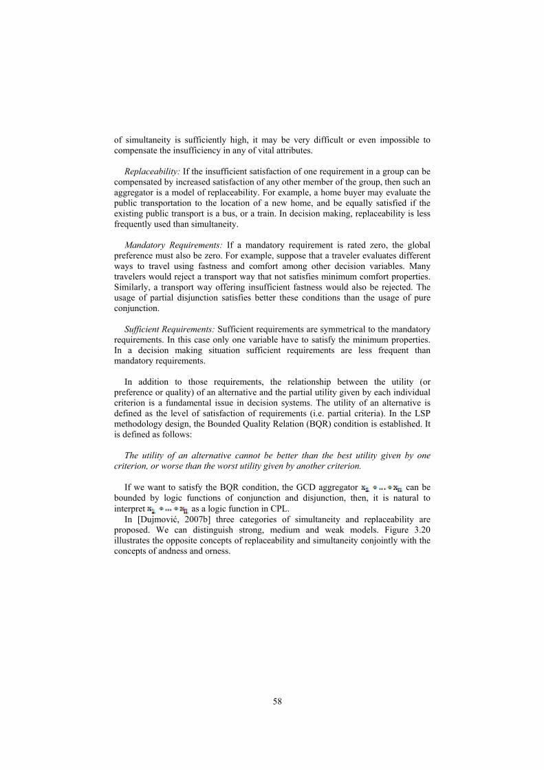
58

of simultaneity is sufficiently high, it may be very difficult or even impossible to compensate the insufficiency in any of vital attributes.

Replaceability: If the insufficient satisfaction of one requirement in a group can be

compensated by increased satisfaction of any other member of the group, then such an aggregator is a model of replaceability. For example, a home buyer may evaluate the public transportation to the location of a new home, and be equally satisfied if the existing public transport is a bus, or a train. In decision making, replaceability is less frequently used than simultaneity.

Mandatory Requirements: If a mandatory requirement is rated zero, the global

preference must also be zero. For example, suppose that a traveler evaluates different ways to travel using fastness and comfort among other decision variables. Many travelers would reject a transport way that not satisfies minimum comfort properties. Similarly, a transport way offering insufficient fastness would also be rejected. The usage of partial disjunction satisfies better these conditions than the usage of pure conjunction.

Sufficient Requirements: Sufficient requirements are symmetrical to the mandatory

requirements. In this case only one variable have to satisfy the minimum properties. In a decision making situation sufficient requirements are less frequent than mandatory requirements.

In addition to those requirements, the relationship between the utility (or

preference or quality) of an alternative and the partial utility given by each individual criterion is a fundamental issue in decision systems. The utility of an alternative is defined as the level of satisfaction of requirements (i.e. partial criteria). In the LSP methodology design, the Bounded Quality Relation (BQR) condition is established. It is defined as follows:

The utility of an alternative cannot be better than the best utility given by one

criterion, or worse than the worst utility given by another criterion. If we want to satisfy the BQR condition, the GCD aggregator can be

bounded by logic functions of conjunction and disjunction, then, it is natural to interpret as a logic function in CPL.

In [Dujmović, 2007b] three categories of simultaneity and replaceability are proposed. We can distinguish strong, medium and weak models. Figure 3.20 illustrates the opposite concepts of replaceability and simultaneity conjointly with the concepts of andness and orness.

59

Figure 3.20 Simultaneity/replaceability related to addness and orness In the case of two input variables , the simultaneity and

replaceability are modeled as functions that generate the aggregated result x y in the following three characteristic regions:

1) Medium models (averaging): ; 2) Strictly strong models: ; 3) Strictly weak models: .

The models that are not strict may include the limit values. Medium and weak

models satisfy the BQR. Strong models do not satisfy the BQR. The operators of medium simultaneity/replaceability (the averaging operators)

have been studied in great detail in Fuzzy Logic and Fuzzy multicriteria decision making. There are several methods in this group from means, in the simplest case, to WPM (used in this approach), and also via other operators like OWA, etc. [Torra&Narukawa, 2005].

Strong models of simultaneity use triangular norms and strong models of replaceability use the corresponding triangular conorms.

Weak simultaneity/replaceability models based on implicative weights were introduced by Larsen [Larsen, 2003].

Several versions of GCD are available in the literature but the most suitable for satisfying the CPL conditions [Dujmović, 2007b] is the Weighted Power Mean (GCD/WPM).

60

 

 

 

 

 

 

 

GCD/WPM is a function that depends on the parameter r. This parameter determines the behavior of the aggregation operator. For , it reduces to the arithmetic mean (neutrality). For it is a partial conjunction (andor,

) and for it becomes the partial disjunction (orand, ).WPM is not symmetrical with respect to the central point r = 1, and this can be used to generate four distinct variants of GCD/WPM (combinations of two forms of andor and two forms of orand in the whole range ).

61

In Table 3.7 we can see the possible values of r depending on the level of polarization of the operators. An explanation of how can be obtained the r values of each operator is available in [Dujmović, 2007b, section V].

Type of polarization

Level of

polarization Symbol d Orness

c Andness

r Exponent

Strongest D 1 0 + ∞ Very Strong D++ 0,9375 0,0625 20,63 Strong D+ 0,875 0,125 9,521 Medium Strong D+- 0,8125 0,1875 5,802

Medium DA 0,75 0,25 3,929 Medium Weak D-+ 0,6875 0,3125 2,792

Weak D-+ 0,625 0,375 2,018

Disjunctive polarization (Partial disjunction)

Very weak D-- 0,5625 0,4375 1,449 Neutrality A 0,5 0,5 1

Very weak C-- 0,4375 0,5625 0,619 Non mandatory Weak C- 0,375 0,625 0,261

Medium Weak C-+ 0,3125 0,6875 -0,148

Medium CA 0,25 0,75 -0,72 Medium Strong C+- 0,1875 0,8125 -1,655

Strong C+ 0,125 0,875 -3,51 Very Strong C++ 0,0625 0,9375 -9,06

Conjunctive polarization (Partial conjunction)

Mandatory requirements

Strongest C 0 1 - ∞

Table 3.7 Logic Scoring Preference operators based in CPL

There are several examples of LSP method in the literature, it is used for evaluation, comparison, selection, and optimization of different elements, such as computers [Dujmović, 2003], data management systems [Su et al.,1987], web sites [Olcina et. Al, 2001], integrated development environments [Dujmović et al., 2006], etc.

There is a commercial software tool that implements the LSP method and its additional analysis tools for making professional evaluation process. It is exploited by SEAS company (http://www.seas.com). SEAS company is specialized in quantitative methods for evaluation, comparison, and selection of complex products or services.

There is no license for academic or research use, so we have implemented the LSP aggregation methodology from scratch using the Analytica tool.

Analytica is other software of Lumina Decision Tools. It is a visual tool for creating, analyzing, and communicating decision models. Some academic license of this software can be bought, so we have used a license available for this research project thanks to the AGA research group. This tool is easy to use and allows you to implement decision systems ad it is used frequently in decision support systems related to environmental and chemical problems due to its implementation of many statistical functions.

62

One of the best things of Analytica is its great graphical interface which facilitates the use of the developed systems for non computer science experts. It can acquire the input data from external files like spreadsheets. Analytica permits to interact with the system visualizing the components of the system and making changes easily and quickly.

3.9. Aggregation of utilities with LSP

As it has been introduced in section before, Analytica is the tool used to implement the aggregation method selected to solve this complex environmental problem. Its main functionality is the graphical representation of the underlying model, which facilitates not only the implementation of the system, but also the use of the system by non experts, such as the decision makers that will use this tool in the future.

The Analytica software is based on building components (nodes) that implement some kind of functionality. Then, the nodes can be linked with arrows to obtain the desired model structure. In Analytica many types of nodes could be used in order to build a decision support system, but to solve this problem only two types of nodes have been used: variables and functions, as well as, arrows that allow to join the different nodes (see Figure 3.21).

The variables can be identified as a rectangle with round corner and they allow to load data from external files using OLE links, i.e. input data can be imported from structured files like spreadsheets (.xls) or files with data separated with comas (.csv). In this problem the importation of data takes place from “.csv” files, that are the output files from the expert systems and the input data explained in section 3.4.5. The variables can also obtain data from other variables, this is possible joining two variables with an arrow and the arrows direction indicates which node receives the data. They use operators like (+, -, x, /) or functions to treat the input data and obtain a result.

On the other hand the functions are represented as “big arrows” and they permit to save a conjoint of operators or other functions in separated structures that can be used to define variables.

Usually the variables that load data from external files don’t have any operator modifying the input data. Other variables take the data from them and use it helped with functions to obtain results.

Figure 3.21 Analytica nodes: Variable, Function

To obtain more information about Analytica, what it is able to do, information

about the different structures, etc, a user manual is available [Analytica, 2009].

63

After this fast introduction to Analytica interface, we are going to explain how is implemented the LSP method and the entire model. First of all, the system has been designed following the structure of the family of criteria. To aggregate the criteria of a lower level to obtain the criteria of a higher level, different aggregation operators have been chosen from the LSP model. A representation of the LSP aggregation has been drawn in Figure 3.22. This figure shows the same criteria hierarchy as in Figure 3.1, it shows the weights used to each criterion and also the aggregation operator used (see Table 3.7) in each aggregation variable, for example soil1 and soil2.

64

Figure 3.22 MCDA Tool model representation

65

In Figure 3.22 the (leaf nodes) represented by ellipses represent complex criteria and the nodes represented by rhomboid represent simple criteria. The nodes represented by rectangles are weights need in the LSP aggregation process and the nodes represented by a polygonal shape represent aggregation nodes. In these nodes the LSP operators are used to calculate the partial / final result utility of each alternative.

In the complex criteria nodes, the utility values are read directly from the files produced by the expert systems files, because these files contains the utility of each alternative calculated from the fuzzy rules. On the other hand, all the simple criteria load the input data about the alternatives’ properties from a single file and then each node use the corresponding utility function (defined in section 3.4.6) to convert the input values into utility values.

Figure 3.23 A simple utility function on Analytica

As it has been showed in section 3.4.6 and Figure 3.3 and in Figure 3.23 the utility functions of simple criteria are quite simples and have defined a piecewise form. They have been implemented with aid of if-then statements and the use of basic operations.

Figure 3.24 shows all the functions implemented in an Analytica library and used on the Analytica project. In the first part there are the LSP operators, in the first row there are the LSP operators with two inputs (and two weights), and in the second row the operators with three inputs. The second part belongs to the utility functions for simple criteria, and the other functions are used to calculate the economical costs.

66

Figure 3.24 Mathematical functions implemented on Analytica

The weights used with each criterion value have been decided jointly with the group of experts, studying the variables involved in each aggregation process and their importance to the result and decision.

A selection of five of the most representative LSP operators has been done in order to facilitate the decision process of which operator is the most appropriated. The LSP operators have been also decided with the help of domain experts. The simultaneity and replaceability degree of the criteria have been the most valued properties in the selection process.

Figure 3.25 shows the hierarchical structure of the criteria model presented over the Analytica software. There is a legend explaining the meaning of the different colors in the figure.

67

Figure 3.25 Decision Making model for biosolid management with Analytica

68

3.10. Flow of execution

After having presented the set of tools in a separate way, the following diagram shows the architecture of the multicriteria decision aid system that has been designed and implemented in this master thesis. Figure 3.26 represents the workflow of the execution process of the different tools.

Figure 3.26 Decision Support System execution flow

Details about the execution of all those stages are explained in the user manual in Annex A:, Data Preparation, execution of the Expert systems over fuzzyTECH and the execution of the LSP method over Analytica.

69

4. Used Data and results

This section explains the experiments that have been done to test the performance of the Multicriteria Decision Aid system developed in this Master Thesis.

Due to the lack of historical data about this problem, because it has not been studied including so much information (for example, previous studies do not consider organic compounds), the collection of data is also one of the tasks done in the research project.

The different research groups on environment involved in the project, Anàlisi i Gestió Ambiental and Laboratorio de edafología, have collected samples of different types of sludge coming from different WWTP, as well as, samples of different types of soils in Catalonia. The construction of the data matrix is explained in this section and the results obtained by the system are also presented and analyzed.

In addition, a sensitivity analysis has been done to evaluate the sensibility of the system if the using weights are modified. It has been impossible to make a sensitivity analysis of the aggregation operators due to lack of time. The results are presented in this section too.

4.1 Data

The data used in this test has been obtained in waste water treatment plants and lands from Catalonian territories. The samples collected have been analyzed in different laboratories (toxicology, chemistry, etc.), in order to obtain the values required to take the decision.

Sludge data has been collected from some plants in the south of Catalonia and others in the north. Due to confidentiality, we cannot give the exact details about those WWTP, however, we include a general description of the characteristics of the sewage sludge they produce (see Table 4.1).

Three types of sludge (industrial, residential or mixed) can be distinguished in the representative samples. The mixed type corresponds to sludge originated in areas with both industrial and residential characteristics.

70

Sludge General Description WWTP1 Mixed sludge WWTP2 Residential sludge WWTP3 Residential sludge WWTP4 Residential sludge

Table 4.1 Table of the WWTP types used to take sludge samples for the test phase

On the other hand, we have the soil data from 6 different soils around Catalonia,

which are briefly described in Table 4.2. The majority of them come from the Tarragona region but there are some of them close to the Catalonian north coast.

Table 4.2 Landscapes types used to take the soil samples in the test phase

The system permits to evaluate simultaneity different sludge over different soils.

Thus, the experiment will include the analysis of the combinations of the 4 WWTP sewage sludge and the 6 different agricultural soils. Consequently, the case study includes 24 alternatives that will permit to study which will be the preference of disposing any sludge at each different soil according their properties at each different agricultural destination. The Table 4.3 identifies the different used alternatives.

Alternatives Description Alternatives Description T1 L1-WWTP1 T13 L1-WWTP3 T2 L2-WWTP1 T14 L2-WWTP3 T3 L3-WWTP1 T15 L3-WWTP3 T4 L4-WWTP1 T16 L4-WWTP3 T5 L5-WWTP1 T17 L5-WWTP3 T6 L6-WWTP1 T18 L6-WWTP3 T7 L1-WWTP2 T19 L1-WWTP4 T8 L2-WWTP2 T20 L2-WWTP4 T9 L3-WWTP2 T21 L3-WWTP4 T10 L4-WWTP2 T22 L4-WWTP4 T11 L5-WWTP2 T23 L5-WWTP4 T12 L6-WWTP2 T24 L6-WWTP4

Table 4.3 Set of alternatives in the case study

Agricultural soil General Description L1 Acid soil, low organic matter and coarse texture L2 Basic soil, high organic matter and medium texture L3 Slightly basic soil, high organic matter and medium texture L4 Natural soil, low organic matter, coarse texture L5 Basic soil, low organic matter, fine texture L6 Acid soil, low organic matter and coarse texture

71

4.2 Evaluate alternatives against criteria

In our proposal, the evaluation of the alternatives is done with the use of fuzzy expert systems for complex criteria and linear utility functions for simple criteria.

In order to assess the utility of each criterion in the system, it has been built a data matrix with the values of the different variables that are related to complex and simple criteria. This data matrix is the input source of the Fuzzy Expert Systems that calculate the utility values of the complex criteria. The data matrix is shown in the following Table 4.5. In this data matrix, each column corresponds to a different variable. The first columns P1 to P9 show the properties of the agricultural soil. The columns P10 to P14 gives data about the population living near the soil and also the distance between the water waste treatment plant and the possible landscape to throw the sludge. Finally, the columns P14 to P20 contain the properties of the sewage sludge. The meaning of the columns is given in Table 4.4.

More details about the construction of this data matrix are given in the ANNEX A, User’s Guide. Property name Abbreviation 1 Abbreviation 2 Soil Texture Soil_Tx P1 Soil Organic Matter Soil_OM P2 Soil pH Soil_pH P4 Soil Nitrates Soil_N P5 Soil Carbon Soil_C P6 Soil DRASTIC Soil_DR P7 Soil Temperature Soil_Te P8 Crop Type Crop_Type P9 Application Type Aplic_Type P10 Population Type Pop_Type P11 Population Density Pop_Dens P12 Distance to Urban Areas Dist_UA P13 Distance WWTP-Land Dist_WWTP P14 Sludge Treatment Type Sludge_TT P15 Sludge Organic Matter Sludge_OM P16 Sludge pH Sludge_pH P17 Sludge Nitrates Sludge_N P18 Sludge Metals Sludge_Me P19 Sludge POPs Sludge_Po P20

Table 4.4 Criteria abbreviations The utility values obtained for each complex criterion can be seen in Table 4.6. The utility scores are in the 0-1 interval. Higher values mean better utility, so more

preferred alternatives.

72

Table 4.5 Data for each input property

P1 P2 P3 P4 P5 P6 P7 P8 P9 P10 P11 P12 P13 P14 P15 P16 P17 P18 P19 P20T1 0 1,11 6,8 10,75 1 45 10 125 agriculture 0 Mid-sensitive 160 7 170 0 45,42 6,91 6,61 0,2 0,2 T2 1 2,34 8,2 10,46 25 33 7,5 125 agriculture 1 Mid-sensitive 430 4 125 0 45,42 6,91 6,61 0,2 0,2 T3 1 2,98 7,7 5,52 25 33 10 75 agriculture 0 Mid-sensitive 163 2 30 0 45,42 6,91 6,61 0,2 0,2 T4 0 0,61 6,9 11,1 1 40 10 75 agriculture 1 Mid-sensitive 163 3 30 0 45,42 6,91 6,61 0,2 0,2 T5 2 1,7 8 9,4 23,2 33 10 100 agriculture 0 Mid-sensitive 135 4 35 0 45,42 6,91 6,61 0,2 0,2 T6 0 0,71 5,6 10,1 0,1 45 10 75 agriculture 0 Mid-sensitive 973 2 135 0 45,42 6,91 6,61 0,2 0,2 T7 0 1,11 6,8 10,75 1 45 10 125 agriculture 0 Mid-sensitive 160 7 170 1 57,7 8,18 4,14 0,5 0,5 T8 1 2,34 8,2 10,46 25 33 7,5 125 agriculture 1 Mid-sensitive 430 4 130 1 57,7 8,18 4,14 0,5 0,5 T9 1 2,98 7,7 5,52 25 33 10 75 agriculture 0 Mid-sensitive 163 2 20 1 57,7 8,18 4,14 0,5 0,5 T10 0 0,61 6,9 11,1 1 40 10 75 agriculture 1 Mid-sensitive 163 3 20 1 57,7 8,18 4,14 0,5 0,5 T11 2 1,7 8 9,4 23,2 33 10 100 agriculture 0 Mid-sensitive 135 4 20 1 57,7 8,18 4,14 0,5 0,5 T12 0 0,71 5,6 10,1 0,1 45 10 75 agriculture 0 Mid-sensitive 973 2 135 1 57,7 8,18 4,14 0,5 0,5 T13 0 1,11 6,8 10,75 1 45 10 125 agriculture 0 Mid-sensitive 160 7 60 1 68,7 6,9 6,06 0,8 0,8 T14 1 2,34 8,2 10,46 25 33 7,5 125 agriculture 1 Mid-sensitive 430 4 110 1 68,7 6,9 6,06 0,8 0,8 T15 1 2,98 7,7 5,52 25 33 10 75 agriculture 0 Mid-sensitive 163 2 235 1 68,7 6,9 6,06 0,8 0,8 T16 0 0,61 6,9 11,1 1 40 10 75 agriculture 1 Mid-sensitive 163 3 235 1 68,7 6,9 6,06 0,8 0,8 T17 2 1,7 8 9,4 23,2 33 10 100 agriculture 0 Mid-sensitive 135 4 240 1 68,7 6,9 6,06 0,8 0,8 T18 0 0,71 5,6 10,1 0,1 45 10 75 agriculture 0 Mid-sensitive 973 2 105 1 68,7 6,9 6,06 0,8 0,8 T19 0 1,11 6,8 10,75 1 45 10 125 agriculture 0 Mid-sensitive 160 7 10 2 56,6 8,4 3,88 0,5 0,8 T20 1 2,34 8,2 10,46 25 33 7,5 125 agriculture 1 Mid-sensitive 430 4 75 2 56,6 8,4 3,88 0,5 0,8 T21 1 2,98 7,7 5,52 25 33 10 75 agriculture 0 Mid-sensitive 163 2 200 2 56,6 8,4 3,88 0,5 0,8 T22 0 0,61 6,9 11,1 1 40 10 75 agriculture 1 Mid-sensitive 163 3 200 2 56,6 8,4 3,88 0,5 0,8 T23 2 1,7 8 9,4 23,2 33 10 100 agriculture 0 Mid-sensitive 135 4 205 2 56,6 8,4 3,88 0,5 0,8 T24 0 0,71 5,6 10,1 0,1 45 10 75 agriculture 0 Mid-sensitive 973 2 50 2 56,6 8,4 3,88 0,5 0,8

73

Groundwater contamination

Groundwater vulnerability

Human Ingestion dose

Human Labor

Soil Biodiversity

Soil Nitrates

Soil Organic Matter

Soil pH Soil Contamination

T1 0.52738 0.5 0.75788 0.20002 0.59664 0.7 0.64998 0.60936 0.80344 T2 0.59998 0.5 0.9 0.40004 0.79998 0.83332 0.7 0.95102 0.79998 T3 0.59998 0.5 0.9 0.20002 0.79998 0.45 0.7 0.96054 0.79998 T4 0.42498 0.5 0.7 0.40004 0.46666 0.7 0.65 0.64704 0.79998 T5 0.69998 0.5 0.875 0.20002 0.77498 0.79998 0.64998 0.93364 0.79998 T6 0.42498 0.5 0.7 0.20002 0.46666 0.69998 0.65 0.60936 0.79998 T7 0.30106 0.4 0.55788 0.40004 0.40666 0.67392 0.7 0.96674 0.37374 T8 0.60344 0.4 0.76666 0.59994 0.74996 0.72762 0.75 0.79996 0.54996 T9 0.60344 0.4 0.7 0.40004 0.74996 0.51798 0.75 0.90006 0.57998 T10 0.25 0.4 0.5 0.59994 0.32 0.67392 0.7 0.9479 0.28332 T11 0.60582 0.4 0.72498 0.40004 0.7 0.82398 0.7 0.85012 0.63634 T12 0.25 0.4 0.5 0.40004 0.32 0.67082 0.7 0.96674 0.28332 T13 0.27166 0.5 0.4 0.40004 0.24666 0.67734 0.7149 0.59994 0.34794 T14 0.44998 0.5 0.7 0.59994 0.55 0.75242 0.75478 0.96674 0.36 T15 0.44998 0.5 0.6 0.40004 0.55 0.50804 0.75478 0.96674 0.35 T16 0.25 0.5 0.4 0.59994 0.225 0.67734 0.70874 0.63326 0.26666 T17 0.47998 0.5 0.56 0.40004 0.52498 0.80432 0.7149 0.967 0.38748 T18 0.25 0.5 0.4 0.40004 0.225 0.6731 0.70874 0.59994 0.26666 T19 0.47546 0.5 0.68384 0.59994 0.42498 0.64456 0.8 0.96674 0.42556 T20 0.55784 0.5 0.82498 0.79996 0.61426 0.70752 0.64998 0.79996 0.56664 T21 0.55784 0.5 0.8 0.59994 0.61426 0.70478 0.64998 0.90006 0.4857 T22 0.32498 0.5 0.59998 0.79996 0.36 0.64456 0.9 0.9479 0.34998 T23 0.58464 0.5 0.7222 0.59994 0.59998 0.8413 0.8 0.85012 0.50766 T24 0.32498 0.5 0.59998 0.59994 0.36 0.66716 0.9 0.96674 0.34998

Table 4.6 Utility values from Expert systems

74

As it has been explained in section 3.4.6, in the complex criteria case, the utilities are obtained from the defuzzification of the conclusions of the fuzzy rules that are activated by each alternative.

For example, in the pH expert system, the ph of the soil and sludge of the alternatives are studied. If we take the alternative L1-WWTP1, it has sludge with a pH value of 6.91 and a soil with a ph value of 6.8. These values activate in the rule block of the expert system the following rules as it is shown in Figure 4.1:

If sludge pH = medium and soil pH = low the utility = 0.6 (0.95 %) If sludge pH = high and soil pH = low then utility = 1 (0.05 %) The first rule concludes that the utility is 0.6 at a degree of 0.95%, whereas the

second one concludes that the utility is 1at a degree of 0.05%. The combination of these two conclusions gives the final utility value 0.6094.

Figure 4.1 Example of pH expert system evaluating alternative 1

In section 3.6.2 other example of the utilities calculation of complex criteria is

given, concretely the evaluation of organic matter expert system is done.

75

Once the utilities of complex criteria have been calculated, the Analytica tool can be used to obtain the utilities for the simple criteria. In this case, the utility is given by a piecewise linear function, since it only depends on a single variable.

For example the utility for the temperature simple criteria following the graphical

representation of the temperature given in section 3.4.6 is as follows: Temperature utility = if temperature >= 20 then 1 else ( ( 5 * temperature ) / 100 ) If we use the first alternative T1 (L1-WWTP1) its temperature input value is 10ºC

the second condition is activated and then: Temperature utility = (5 * 10)/100 = 0.5 Table 4.7 shows all the utilities calculated with this process for this case study, we

can check that the obtained temperature value is the same that there is in the table. Soil

temp. Crop type

Population type

Populationdensity

Precip. Distance to urban areas

Fertilizer reduction cost

Transport cost

Storage cost

T1 0.5 0.9 0.6 0.85 0.14 0.019 0.5 0.52 0.40 T2 1 0.9 0.6 0.58 0.14 0 0.5 0.52 0.40 T3 0.5 0.9 0.6 0.85 0.07 0 0.5 0.72 0.40 T4 0.5 0.9 0.6 0.85 0.07 0 0.5 0.72 0.40 T5 0.5 0.9 0.6 0.87 0.10 0 0.5 0.72 0.40 T6 0.5 0.9 0.6 0.027 0.07 0 0.5 0.52 0.40 T7 0.5 0.9 0.6 0.85 0.14 0.019 0.5 0.7 0.40 T8 1 0.9 0.6 0.58 0.14 0 0.5 0.7 0.40 T9 0.5 0.9 0.6 0.85 0.07 0 0.5 0.825 0.40 T10 0.5 0.9 0.6 0.85 0.07 0 0.5 0.825 0.40 T11 0.5 0.9 0.6 0.87 0.10 0 0.5 0.825 0.40 T12 0.5 0.9 0.6 0.027 0.07 0 0.5 0.7 0.40 T13 0.5 0.9 0.6 0.85 0.14 0.019 0.5 0.763 0.40 T14 1 0.9 0.6 0.58 0.14 0 0.5 0.7 0.40 T15 0.5 0.9 0.6 0.85 0.07 0 0.5 0.7 0.40 T16 0.5 0.9 0.6 0.85 0.07 0 0.5 0.7 0.40 T17 0.5 0.9 0.6 0.87 0.10 0 0.5 0.7 0.40 T18 0.5 0.9 0.6 0.027 0.07 0 0.5 0.7 0.40 T19 0.5 0.9 0.6 0.85 0.14 0.019 0.5 0.91 0.91 T20 1 0.9 0.6 0.57 0.14 0 0.5 0.87 0.91 T21 0.5 0.9 0.6 0.85 0.07 0 0.5 0.84 0.91 T22 0.5 0.9 0.6 0.85 0.07 0 0.5 0.84 0.91 T23 0.5 0.9 0.6 0.87 0.10 0 0.5 0.84 0.91 T24 0.5 0.9 0.6 0.027 0.07 0 0.5 0.87 0.91

Table 4.7 Utility values from simple criteria

76

4.3 Rating and evaluation of results

Now, all the utilities are known and the aggregation can be done. As the LSP method makes partial aggregations at different levels, the partial ratings can also be studied. The parameters used have been explained at section 3.9 (i.e. weights and conjunctive/disjunctive operators). They have been defined by the environmental experts. The following figures (from Figure 4.3 To Figure 4.14) shows the results at each different aggregation node of the model. The hierarchical structure of the model is shown again in the Figure 4.2.

The rest of bar diagrams show the degree of suitability of the alternative with respect to each criterion. The ratings are in the 0-1 interval, the higher the value, the better is the use of that sludge in that soil with respect to the criterion evaluated.

77

Figure 4.2 MCDA Tool model representation

78

Figure 4.3 Results of soil1 aggregation node

In the aggregation node soil1 (Figure 4.3), three simple criteria are aggregated:

organic matter, pH and nutrients. Rating these three soil properties we can observe than the best alternative is the T23, corresponding to the L5 and WWTP4. As we will see in the following pictures, altogether, the alternatives with sludge from the WWTP4 usually have very good ratings. But in this case alternative T23 is followed closely by alternative T2 composed by L2 and WWTP1. These two alternatives have an equal characteristic, they are basic soils. On the other hand the worst alternative is the T3 (L3-WWTP1).

Figure 4.4 Results of soil2 aggregation node

79

In the soil2 node (Figure 4.4), that aggregates the utilities from the biodiversity and

the soil contamination complex criteria, we can observe so much differences between the ratings of each alternative, and in this case it seems that in general alternatives w WWTP1 Sludge have better values than alternatives with WWTP2 sludge and so on, to reach the worst alternatives that use WWTP3 and after better values are observed in alternatives with WWTP4.

There are two alternatives with the best rating, T2 (L2-WWTP1) and T3 (L3-WWTP2) and the worst alternatives are T16 (L4-WWTP3) and T18 (L6-WWTP3).

Figure 4.5 Results of groundwater aggregation node

In ground water node (Figure 4.5)the utilities from the ground water vulnerability

and ground water contamination criteria are aggregated. In this case it is observable that for each group of alternatives that use the same sludge, there are relatively high variations between their ratings. The alternatives that use WWTP2 sludge are a clear example.

In this graphic the best alternative is T5 (L5-WWTP1) and the worst are T10 (L4-WWTP2) and T12 (L6-WWTP2).

80

Figure 4.6 Results of population aggregation node

The population node (Figure 4.6) aggregates the utilities from population type,

population density and distance to urban areas simple criteria related to human health properties. As it is observable these three alternatives do not have any relation with any sludge property and as a consequence in this case we can see that the alternatives have the same values for each soil. There is not a clear winner in this case, the best place is for L5 (T5, T11, T17, T23), but it obtains a quite similar evaluation that L1, L3 ad L4. On the other hand the worst alternatives use L6 soil (T6, T12, T18, T24). L2 has also quite poor evaluations compared with the best ones.

Figure 4.7 Results of landscape aggregation node

81

The entire alternative ratings of the landscape node (Figure 4.7) are almost equal, all alternatives have utilities close to 0.8. This alternative aggregate the utility values from precipitation, temperature and crop type simple criteria, in this case the alternatives are also related only with soil properties, for this reason the alternatives that use the same soil have the same evaluation.

The worst alternatives are T2, T8, T14, and T20, they use S2. The other alternatives have the same ratings, the best one.

In fact, in this case study, we can see that this criterion does not permit to decide upon the alternatives. This indicates that it should be studied in more detail if it should be included in the decision model or it can be removed from it. A more exhaustive testing is needed to see whether the landscape is important or not.

Figure 4.8 Results of soil aggregation node

In the soil aggregation node (Figure 4.8), two previous aggregated values are

considered: soil1 and soil2. In this case the best alternative is T2 (L2-WWTP1) followed by T5 (L5-WWTP1) and the worst alternative are T16 (L4-WWTP3) and T18 (L6-WWTP3). This situation is very similar to the situation of soil2 node, where we have the same worst nodes and T2 is not the better bat is the second one.

On the other hand, it is interesting to see that alternatives that use L5 have very good ratings if they are compared with the alternatives that use the same sludge.

82

Figure 4.9 Results of population risk aggregation node

Very similar ratings are observed in the population risk node (Figure 4.9). This

node aggregates the population and landscape nodes. Similarly to the two cases studied the ratings are the same for the alternatives that use the same sludge. The alternatives that use L5 soil have the best ratings and on the other hand the alternatives that use L2 soil have the worst ones. This situation is similar to the last node analyzed where the alternatives with L5 soil had very good ratings.

However, we can see that the aggregation of the landscape (Figure 4.7)evaluation (which was a value of 0.8 for all the alternatives) to the population has the effect of reducing the differences between the alternatives that were observed in the population criterion (Figure 4.6). In fact, although both elements have the same weight, the aggregation operator used in this case is the one denoted by DA in Table 3.7, which is a disjunctive operator. That means that if one of the two criteria has a high value, this is enough to give a high result. In this case, the use of this disjunctive operator must be reviewed with the experts to see if it is appropriate.

83

Figure 4.10 Results of exposure risk aggregation node

The better ratings for the exposure risk node (Figure 4.10), in general, are observed

from alternatives that use WWTP4 sludge, on the other hand the worst ratings come from alternatives with WWTP1 sludge, which is classified as mixed; i.e. it comes from an industrial and residential region. The exposure risk node aggregate utilities from population risk node and labor simple criteria.

In this case the best alternative is T22 (L4-WWTP5) and the worst is T6 (L6-WWTP1).

Figure 4.11 Results of economical aggregation node

84

In the economical node (Figure 4.11) there are some clear winners, the alternatives with WWTP4 sludge have the best ratings, on the other hand the worst alternatives use WWTP1 sludge.

This node aggregates the three economical and simple criteria, transport cost, storage cost and fertilizer reduction cost.

In more detail we can see that alternative T19 (L1-WWTP4) is the best one and alternatives T1 (L1-WWTP1), T2 (L2-WWTP1) and T6 (L6-WWTP1) are the worst.

Figure 4.12 Results of environmental risk aggregation node

The environmental node (Figure 4.12) aggregates the utilities from the soil and the

groundwater nodes. This node is the last step in the hierarchy including all environmental properties involved in the system.

In this node the best rating is obtained by alternative T5 (L5-WWTP1) and the worst rating is had by alternatives T16 (L4-WWTP3) and T18 (L6-WWTP3). It is a situation very similar to the soil node. In this case the alternatives with L5 have better results than the alternatives hat use the same sludge and they highlight from their neighbors (alternatives with L4 or L6 soil).

85

Figure 4.13 Results of human health risk aggregation node

The human health risk node (Figure 4.13) aggregates the exposure risk node with

the ingestion dose simple criteria. This node includes all the properties that could affect the human health.

In this graphic we can observe, in general, that the alternatives with WWTP4 sludge are the best and alternatives with WWTP3 sludge are the worst. More concretely the best alternative is T20 (L2-WWTP4) and the worst are T13 (L1-WWTP3), T16 (L4-WWTP3) and T18 (L6-WWTP3).

Figure 4.14 Results of general evaluation aggregation node

86

Finally we have arrived to the general evaluation node (Figure 4.14), the node that offers us the final utility ranking of alternatives. As we have been explaining on partial assessments, in general the alternatives with WWTP4 sludge have the better ratings, on the other hand the alternatives with WWTP3 have the worst ones.

In this case we can say that the best alternative is T20 (L2-WWTP4) and the worst is T18 (L6-WWTP3).

In the following table (see Table 4.8) the best and the worst alternatives for each type of sludge are represented. In the table we are able to see that S6 soil is the worst option for every studied sludge and S2 soil is the best in the majority of cases. Best soil Next good options Worst soil WWTP1 L2 (0.606) L5 (0.592) - L4 (0.588) L6 (0.514) WWTP2 L5(0.619) L2 (0.609) - L3 (0.604) L6 (0.454) WWTP3 L2(0.578) L5 (0.557) - L3 (0.551) L6 (0.418) WWTP4 L2(0.606) L5 (0.68) - L3 (0.672) L6 (0.566)

Table 4.8 Ranking of soils with respect to WWTP sewage sludge This table is very interesting and useful for the decision maker that has to manage

the sewage sludge application on those soils. Considering that a single soil must be assigned to each sludge, a reasonable decision could be the next one:

• WWTP1 sludge is sent to L4, because it permits a degree of suitability of 0.588, only slightly inferior to the best possibility for this sludge.

• WWTP2 sludge is sent to L5, because it is the best option, with a utility value of 0.619.

• WWTP3 sludge is sent to L2, because this is the best option for this sludge, reaching a value of 0.578,

• WWTP4 sludge is sent to L3, because this is the sludge that produces better evaluations with all the soils, and the three best options have all very good ratings. This option is evaluated with a 0.672.

We can conclude saying that the results obtained have been satisfactory. After an

initial evaluation of these results, the experts affirm that their expected results were very similar to the results obtained.

4.4 Validation

Parameter uncertainty is one of the most discussed areas in MCDA, where sensitivity and robustness studies are employed to understand the effects of the parameter variations on the results. Sensitivity analysis and robustness evaluation are regarded as key stages in discrete MCDA where the DM is able to explain the results and make the recommendations with confidence.

As it has been previously defined, the sensitivity analysis is focused on the

studying the impact of the changes on the values, while the robustness analysis

87

evaluates if the results are valid in all or most versions, a version being a possible set of values for the data of the problem and for the parameters of the method [Vincke, 1999].

Although specific methods for robustness analysis are centered on comparing the results of the MCDA model with respect to uncertainty in input data or in different versions of the problem, we can also obtain some robustness conclusions from the sensitivity analysis results, in the sense that if a solution does not depend on the input values, it is robust for all these parameters versions.

4.5 Sensitivity Analysis

The sensitivity analysis studies the effect of the parameters of the LSP method in the results. To make this analysis, we have considered the case study presented in section 4.1, consisting in 24 alternatives, corresponding to different scenarios where the application of sewage sludge of 4 different WWTP against 6 different agricultural soils is evaluated.

The Analytica software has been used to perform this analysis. It includes tools to define probability distributions and methods for sampling, which will be explained later.

To perform the calculation, the model is divided in 5 levels, as shows Figure 4.15. Each of them corresponds to the aggregation of a subset of criteria at different degree of generality. Each box corresponds to the application of an LSP aggregation operator. Each operator has two parameters:

The weights of the criteria: giving the importance of each criterion in the decision Conjunction/disjunction degree: expressing the aggregation policy, enhancing the

simultaneity or replaceability of the different criteria at each particular step.

88

Figure 4.15 Levels in the sensitivity analysis.

The sampling size is 30. This means that the rank is calculated for 30 different sets

values for the parameters for each of the 24 scenarios. Each aggregation operation has been studied separately, starting from the most general aggregation (level I) to the most specific (level V).

The results show the ranking of the alternatives obtained with each different set of values. A tolerance threshold of 2 positions has been considered as acceptable, that is, if the alternative is only placed 2 positions up or down with respect to the different rankings, the result is considered stable.

4.5.1. Sensitivity with respect to the weights

When using a multiattribute utility model for the selection of a preferred alternative the result depends in part on the weighting of the attributes. Since the determination of weights is not easy for the experts, it is appropriate to justify the decision by showing that it is insensitive to weight imprecision [Jessop, 2004].

The sensitivity analysis with respect to the weights given to the criteria before their

aggregation is performed converting the static weights, w, into a normal probability distribution, W, of the following form:

W= N(w,0.1w) This distribution has the center in the initial weight given by the domain experts, w.

Then a deviation of a 10% from this weight is considered. For example, W_human health risk= N(0.4, 0.04) W_environmental= N(0.4, 0.04)

89

W_economical= N(0.2, 0.02) The sample method used is Median Latin Hypercube and the Randomize method is

known as Minimal standard. Then, the obtained W values are normalized such that the following property is

fulfilled (W_norm boxes) for each aggregation operator. ΣWi = 1 The architecture of the sensitivity analysis system developed for performing the

sensitivity analysis at Level I (General evaluation) is shown in Figure 4.16.

W_Humanhealth risk

W_Environmental

GeneralEvaluationW_Economical

Rank

W_norm

W_HH_n

W_ECO_n

W_ENV_n

Figure 4.16 Scheme of the calculation for Level I: General evaluation

4.5.2. Results of the weights sensitivity analysis

In this section, the results are graphically presented for each level. The diagram

shows the position in the ranking obtained by each of the 24 scenarios (T1 … T24) in the 30 different value samples considered. The alternative placed at position 1 is the best one, while the one positioned at place 24 is the worst one.

Remember that according to the case study definition, the first 6 scenarios correspond to the analysis of the sludge coming from WWTP1, the next 6 ones correspond to the sludge from WWTP2 and so on.

90

Level I: General evaluation

Figure 4.27 Results of general evaluation sensitivity analysis

The results (see Figure 4.17) show that the ranking is very stable with respect to the best and worst positions. This means that the best and worst alternatives are clearly established and do not depend on the weights selection (up to the extent of a 10% variation).

The best option is T20 and the second one in T23. They order is only reversed in one case. The third place is always for T31 and the forth for T19, whereas the worst option is T18.

With respect to the intermediate positions, we can see some changes in the ranking depending on the weights selection. For example, T2 and T8, change their relative position (both correspond to the same soil). This means that depending on the weights, the sludge evaluation for this soil changes. The same happens with the alternatives T8 and T11 that correspond to the same Sewage Sludge, depending on the weights selection, the evaluation of this sludge with respect to these two different soils gives a different value leading to a different ranking.

Regardless of these changes, we can see that for the sludge of WWTP1 (T1 .. T6) the best place is alternative is T2 (L2). For sludge of WWTP2 (T7 .. T12) the best place is clearly T11 (L5). For sludge from WWTP3 (T13 .. T18) the best option is T14 (L2). Finally, for WWTP4 (T19 .. T24) the alternative T20 (L2) is the best one, and also the best combination from all.

This stability analysis could help the decision maker to better decide the destination of the sewage sludge depending on the impact of the weights in the ranking.

91

Level II a: Human health risk

Figure 4.38 Results of human health risk evaluation sensitivity analysis

In this case (see Figure 4.18), we also observe that the initial and final positions are clearly defined. Best option: T20, Worst option: T18. In this case, the alternatives in the worst positions should be clearly avoided due to the human health risk that they involve. Moreover, some alternatives obtain quite different positions in the ranking, such as T10 or T12, which will be analyzed by the experts.

In addition, some rank reversals can be found between pairs of alternatives (T2 with respect to T22 and T8 with respect to T19). This indicates that the set of weights has an influence on these particular alternatives, which produces a change in the ranking. This situation will be studied in detail with the environmental experts in the next months.

92

Level II b: Economic

Figure 4.49 Results of economic sensitivity analysis

Due to the restrictions on privacy we cannot give a detailed analysis of the results.

However, we can say that the best values depend on the distance between the WWTP and the agricultural soil. The shortest distances obtain better values than the longest ones.

In this case (see Figure 4.19), the weights have no effect in the ranking, which give the same position always.

We also observe that some sets of alternatives obtain the same evaluation value, which make them be placed to the same position in the ranking (ties).

The economical impact is evaluated considering three criteria with the following initial weights:

Fertilizer reduction cost: 0.2 Transport cost: 0.4 Organic matter weight: 0.4

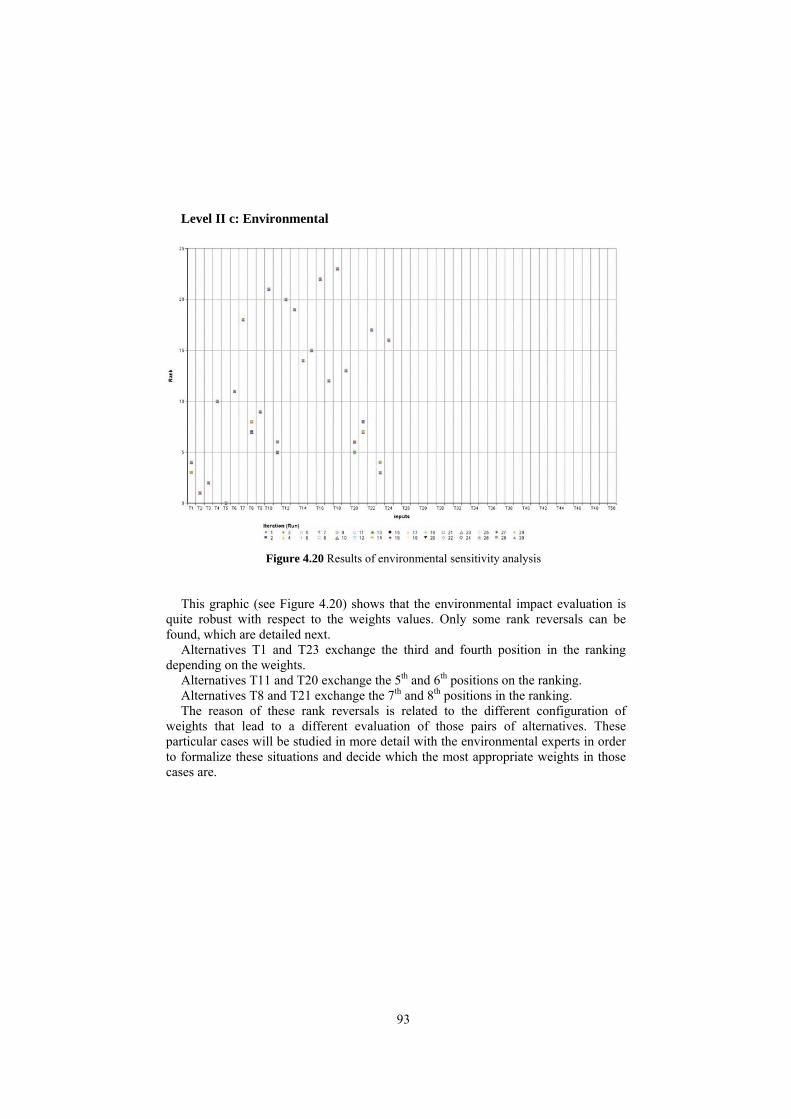
93

Level II c: Environmental

Figure 4.20 Results of environmental sensitivity analysis

This graphic (see Figure 4.20) shows that the environmental impact evaluation is quite robust with respect to the weights values. Only some rank reversals can be found, which are detailed next.

Alternatives T1 and T23 exchange the third and fourth position in the ranking depending on the weights.

Alternatives T11 and T20 exchange the 5th and 6th positions on the ranking. Alternatives T8 and T21 exchange the 7th and 8th positions in the ranking. The reason of these rank reversals is related to the different configuration of

weights that lead to a different evaluation of those pairs of alternatives. These particular cases will be studied in more detail with the environmental experts in order to formalize these situations and decide which the most appropriate weights in those cases are.

94

Level III a: Exposure risk

Figure 4.21 Results of exposure risk sensitivity analysis

In Figure 4.21, the alternatives with best values with respect to the “Exposure risk”

are more sensible to the weights values than the ones with worse values. That is, the first positions in the ranking change depending on the configuration of the weights, see alternatives T19, T20 and T23. Whereas the alternatives in the positions number 8 until position 24 keep insensible to the weights changes.

In particular, the changes in the ranking happen with the evaluation of the sludge from WWTP4. In this case the characteristics of the sludge make it more sensible to the weight configuration in order to decide which the best soil for this sludge is. In any case, the application of this sludge into a soil is always the one with less exposure risk in this case study.

95

Level III b: Soil

Figure 4.22 Results of soil sensitivity analysis

In Figure 4.22, the alternatives with best values with respect to the “Soil” are more sensible to the weights values than the ones with worse values. Whereas the alternatives in the positions number 10 until position 24 keep insensible to the weights changes. Moreover, there are two alternatives that are quite sensible to the weights configuration (T9 and T23). These cases will be analyzed in the detail by the experts.

96

Level III c: Ground Water

Figure 4.23 Results of groundwater sensitivity analysis

In this case (see Figure 4.23), there are three alternatives that are quite sensible to the weights values (T9, T10 and T11). Others remain all ways in the same position, like the best ones (from position 0 to position 6). Finally, some of them have a change of two positions from one ranking to the other. These cases will be studied in the future.

97

Level IV a: Population risk

Figure 4.24 Results of population risk sensitivity analysis

In this case (see Figure 4.24), the weights have no effect in the ranking, which give

the same position always. We also observe that some sets of alternatives obtain the same evaluation value,

which make them be placed to the same position in the ranking (ties). In fact, the ranking only distinguishes 5 positions. It is also worth to note that the position is mainly influenced by the soil and landscape properties rather than the sludge. In fact, this criterion is built without considering sludge properties.

98

Level IV b: Soil 1

Figure 4.25 Results of soil1 sensitivity analysis

In this case (see Figure 4.25), the results show a great sensibility to the weights values. In an initial analysis, the experts proposed to change the weights given to the 3 criteria (nitrates, pH and organic matter). The following table (Table 4.9) shows the initial weights and the proposed ones:

Criterion Initial weight New weight pH 0.1 0.2 Organic matter 0.3 0.3 Nitrates 0.6 0.5

Table 4.9 Initial weights and proposed weights for criteria of soil1 node The purpose is to increase the importance of the pH and decrease the one of the

nitrates, which had a too high influence in the ranking. This proposal will be discussed with the rest of the partners of the project in the next meeting.

99

Level IV c: Soil 2

Figure 4.26 Results of soil2 sensitivity analysis

The second soil sub-criterion exhibits a more robust behavior (see Figure 4.26). The initial positions in the ranking are stable, on only slight changes in the positions of some alternatives are observed.

100

Level V a: Population

Figure 4.27 Results of population sensitivity analysis

The behavior of this criterion (see Figure 4.27) has been explained in the previous level with the more general criterion Population Risk.

101

Level V b: Landscape

Figure 4.28 Results of landscape sensitivity analysis

The behavior of this criterion (see Figure 4.28) has been explained in the previous

level with the more general criterion Population Risk.

102

5. Conclusions and future work

In this Master Thesis we have designed and developed a decision support system for the appropriate application of WWTP sewage sludge in agricultural soils.

To conduct this work, several goals were formulated and now we can say that they have been completely fulfilled:

1. The state of the art in MCDA technologies has been studied in detail, making

an exhaustive search in the literature.

2. The result of this analysis has helped to determine the most appropriate model for the problem considered. In this way the problem has been approached with the Multi-Attribute Utility Theory using numerical and linguistic data and integrating the advantages of rule-based systems and fuzzy logic.

3. I have participated in the knowledge engineering process together with the environmental experts in order to define the decision model (criteria, alternatives, goals, requirements …). Each month we have been met with all experts involved in the project in order to proceed with the project and achieve the goals. The meetings to decide the hierarchical criteria structure have been a hard and long task but finally fructifying. And it is important to remark that the collaboration of each member has made possible the elaboration of the final decision.

4. After studying the existing software tools, none of them was appropriate for the complex decision model that we were designing, so an ad-hoc tool has been implemented. Two commercial tools have been used, fuzzyTECH and Analytica, because groups involved in the project already had licenses of these software, and some experience in their use. A user manual has been written in order to help in the utilization of the decision support system developed.

5. Finally, a case study has been defined and tested. In addition, a sensitivity analysis on the weights has been done. Although this has been quite a brief analysis, it has brought to light many interesting issues that will be further studied by the experts

103

Considering the performed research, the developed methodologies and the obtained results, we can extract the following conclusions:

- Several decision aid tools are available nowadays, and others are in development. The most popular tools have been classified and categorized upon their characteristics. I would highlight the interest of an open source tool, Decision deck, that wants to be a powerful tool with repository of the most popular methods used in decision aid. This is a project under development.

- The great amount of factors involved and interrelated in the problem studied has made difficult the MCDA model definition. Finally, it has been necessary to use two different methodologies for utility assessment and the use of hierarchical aggregation operators to model different levels of criteria. In particular, fuzzy rules have been used to deal with uncertainness and the interrelation between properties, and the LSP method (based on complex logical operators) to aggregate the utilities of the hierarchical criteria structure.

- The analysis of the results done confirms that the approach taken can help the decision makers to find the best agricultural soils for a certain sewage sludge. The results and sensitivity analysis has brought to light some interesting issues regarding the relation between the different sets of criteria, the most suitable weights and the critical values to be considered.

- The work made has a great interest from a practical point of view, but it has also been attracted the attention of the research community. This work has been presented in two conferences and it was invited to participate in the first issue a forthcoming journal specialized in MCDA. It is now in reviewing process. This publications are the following ones:

- M. Schuhmacker, A. Valls, J. Pijuan, A., Passuello, M. Nadal, Multicriteria analysis to manage sewage sludge application on agricultural soils, 19th Annual Meeting of the Society of Environmental Toxicology and Chemistry (SETAC-Europe), Goteborg (Sweden), 2009.

- Valls, A., Shuhmacher, M., Pijuan, J., Passuello, A., Martí, N., Some approaches to the use of MCDA tools for the management of sewage sludge application on agricultural soils, 69th Meeting of the EURO Working Group on Multiple Criteria Decision Aiding, pp. 10-11, Brussels (Belguim), 2009.

- Valls, A., Shuhmacker, M., Pijuan, J., Passuello, A., Martí, N., Sierra, J., On the utility assessment for managing sewage sludge application on agriculatural soils, Submitted to the International Jorunal of Multiple Criteria Decisión Making.

104

As future work we would like to indicate the following research lines:

- The problem studied is a part of a bigger problem where the destination of a sludge that has to consider three possibilities: to be deposited in a landfill, to be incinerated in a cement plant as a combustible or to be used a fertilizer in agricultural landscapes. The adaptation of the actual model to the new problem is one of the first things to do.

- On the other hand, in this work any restrictive law has been taken into account in the criteria, we have assumed that a preprocess has been done eliminating the unsuitable alternatives. For example, it is forbidden the utilization of sludge with a high level of metals concentration. This type of restrictions has to be considered if other destinations, besides the agricultural soil, are considered.

- Another of the goals of this funded research project is to represent the possible destination in maps using geo-positioning. This task is currently in process and it is interesting to study the integration of the decision tool that we have developed with the geo-positioning tools.

- A deeper analysis of the MCDA model with more data will help the experts to write a set of recommendations for decision makers that could be used in a more general level (Spain or even Europe).

Finally, as a personal experience, I would like to affirm that working in a group of people with different background is not easy. One of the reasons is because everybody considers a problem according its point of view and usually it is different from the other and this fact is the cause of misunderstandings. But as a consequence everyone have to make an effort to explain its thoughts in a rough form to be understood, it is a big effort but really, it is a pleasure work with people with different skills because finally you learn a lot, you wins a lot of knowledge and for me the most important, you learn to interpret things from different point of views. I am delighted to have worked with this group as professional and charming.

105

6. Bibliography

[Aller et al., 1987] Aller, L., Bennett, T., Jehr, J.H., Petty R.J. and Hackett G., “DRASTIC: a standardized system for evaluating ground water pollution potential using hydrogeologic settings”. United States Environmental Protection Agency, 622 pp., 1987.

[Analytica, 2009] The Analytica User's Guide, http://analyticaonline.com/ana/Tutorial4_1_1.pdf, 2009.

[Bana , 1990] Bana e Costa, C.A., “Readings in multiple criteria decision aid”. Springer-Verlag, Berlin, 1990.

[Banzhaf, 1965] Banzhaf, J.F., “Weigthed voting doesn't work: A mathematical analysis”, Rutgers Law Review, v.19:2, pp. 317-343, 1965.

[Boettcher&Levis, 1981] Boettcher, K. L., Levis A. H., “Modeling the interacting Decision Maker with bounded rationality”. LIDS-P; 1110, 1981.

[Chen&Klein, 1997] Chen, Ch, Klein, C.M., “An efficient approach to solving fuzzy MADM problems”, Fuzzy Sets and Systems, vol.88, pp.51-67, 1997.

[Dujmović et al., 2008] Dujmović, J. J., De Tré, G., Van de Weghe, N., “Suitability Maps Based on the LSP Method” Lecture Notes on Artificial Intelligence, vol. 5285, pp. 15-25, Springer, 2008.

[Dujmović, 2003] Dujmović J. J., “Optimizing computer system configurations,” Autom. Control, vol. 13, no. 2, pp. 23–33, 2003.

[Dujmović et al., 2006] Dujmović J. J. and Nagashima H., “LSP method and its use for evaluation of java IDE’s”. Int. J. Approx. Reas., vol. 41, no. 1, pp. 3–22, 2006.

[Dujmović, 2007a] Dujmović, J. J., “Properties of Local Andness/Orness”. Theor. Adv. and Appl. of Fuzzy Logic, ASC 42, pp. 54–63, Springer, 2007.

[Dujmović, 2007b] Dujmović, J. J., “Continuous Preference Logic for System Evaluation”. IEEE Transactions on fuzzy Systems. Vol. 15. No 6. December 2007

[Dujmović et al, 2007] Dujmović, J. J. and Larsen H. L., “Generalized conjunction/disjunction,” Int. J. Approx. Reas. 46, pp. 423–446, 2007.

[Dyer, 2005] Dyer, J.S. “MAUT – Multiattribute utility theory”, Multiple Criteria Decision Analysis. State of the art surveys, pp.265-295, Springer, 2005.

[Figueira et al., 2005] Figueira, J., Greco, S., Ehrgott, M., (EDs), “Multiple criteria decision analysis. State of the art Surveys”, Springer, 2005.

106

[Fuentes et al., 2007] Fuentes, J. S., S. F.C., “Resultats de l'aplicació reiterada de fangs d'EDAR en els cultius del cereal”. IRTA Mas Badia Consorci Costa Brava: 13, 2007.

[Fülöp, 2005] Fülöp, J. “Introduction to Decision Making Methods”. Laboratory of Operations Research and Decision Systems, Computer and Automation Institute, Hungarian Academy of Sciences, 2005.

[FuzzyTech, 2009] FuzzyTech software: http://www.fuzzytech.com, September, 2009.

[Giove et al., 2009] Giove, S., Brancia, A., Satterstrom, K., Linkov, I., “Decision Support Systems and Environment: Role of MCDA”. Decision Support Systems for Risk-Based Management of Contaminated Sites, Springer US, 1-21, 2009.

[Grabish&Labreuche, 2005] Grabish, M., Labreuche, C. “Fuzzy measures and integrals in MCDA”, Multiple Criteria Decision Analysis. State of the art surveys, pp.563-608, Springer, 2005.

[Greco et al., 2001] Greco, S., Matarazzo, B., Słowiński, R.: “Rough sets theory for multicriteria decision analysis”. European Journal of Operational Research, 129, 1, 1-47, 2001.

[Greco et al., 2005] Greco, S., Matarazzo, B., Słowiński, R.: “Decision rule approach”. In: Figueira J., Greco S. Ehrgott M.(eds.), Multiple criteria decision analysis: State of the art surveys. Springer, pp 507-563, 2005.

[Henig&Buchanan, 1996] Heing, M., Buchanan, J., “Solving MCDM problems: process concepts”, Journal of multi-criteria decision analysis, vol.5, pp.3-21, 1996.

[van Herwijnen et al., 1993] van Herwijnen, M., Rietveld, P., Thevenet, K., Tol, R., “Sensitivity Analysis with interdependent Criteria for Multicriteria Decision Making. The case of soil Pollution Treatment” Serie Research Memoranda, 1993.

[Janssen, 2001] Janssen, R., “On the use of multi-criteria analysis in environmental impact assessment in the Netherlands”. Journal of Multi-Criteria Decision Analysis 10:101–109, 2001.

[Jensen et al, 2006] Jensen, J., Mesman, J., “Ecological risk assessment of contaminated land - Decision support for site specific investigations”, report 711701047, RIVM, 2006.

[Jessop, 2004] Jessop, A., “Sensitivity and robustness in selection problems”. Computers and Operational Research, vol.31, pp.607-622, April 2004.

[Kaliszewski, 2006] Kaliszewski, I., “Soft Computing for Complex Multiple Criteria Decision Making”, Springer, 2006.

[Kangas et al., 2001] Kangas, J., Kangas, A., Leskinen, P., Pykalainen, J., “MCDM methods in strategic planning of forestry on state-owned lands in Finland: Applications and experiences”. Journal of Multi-Criteria Decision Analysis 10:257–271, 2001.

107

[Kenny&Raiffa, 1993]Keeney, R.L., and Raiffa, H., “Decision with Mutlitple Objectives: Peference and value trafeoffs”. Cambridge University Press, New York, 1993.

[Kiker et al., 2005] Kiker, G. A., Bridges, T. S., Varghese, A., Seager, T. P., Linkov, I., “Application of Multicriteria Decision Analysis in Environmental Decision Making”, Integrated Environmental Assessment and Management, Volume 1, Number 2, pp. 95–108, SETAC, 2005.

[Klir&Yuan, 1995] Klir, G.J. and Yuan, B., “Fuzzy Sets and Fuzzy Logic. Theory and Applications”. Prentice-Hall, 1995.

[Linkov et al., 2005] Linkov I., Kiker, G., Bridges, T., Figueira J., “MCDA and Environmental Problems”, European Working Group Multiple Criteria Decision Aiding, Series 3, nº 12, Fall, 2005.

[Linkov et al., 2004] Linkov, I., Varghese, A., Jamil, S., Seager, TP., Kiker, GA., Bridges, TS., “Multi-criteria decision analysis: Framework for applications in remedial planning for contaminated sites”. In: Linkov I, Ramadan A, editors. Comparative risk assessment and environmental decision making. Amsterdam, The Netherlands: Kluwer. p 15–54, 2004

[Larsen, 2003] Larsen, H. L., “Efficient andness-directed importance weighted averaging operators,” Int. J. Uncertainty, Fuzziness Knowl.-Based Syst., vol. 12, pp. 67–82, 2003.

[Marichal&Roubens, 2000] Marichal, J. L., Roubens, M., “Entropy of discrete fuzzy measures”, International Journal of Uncertainty, Fuzziness and Knowledge Based Systems, v.8:6, pp.625-640, 2000.

[McCarl&Spreen, 2002] McCarl, B. A., Spreen, T.H., “APPLIED MATHEMATICAL PROGRAMMING USING ALGEBRAIC SYSTEMS”, Department of Agricultural Economics, Texas A&M University,2002.

[Mendoza et al., 2002]Mendoza, G. A., Anderson, A.B., Gertner, G.Z.. “Integrating multi-criteria analysis and GIS for land condition assessment: Part 2—Allocation of military training areas”. Journal of Geographic Information and Decision Analysis 6:17–30, 2002.

[Olcina et al., 2001] Olcina, L., Lafuente, G., Rossi, G., “Specifying quality characteristics and attributes for websites”, in Lecture Notes in Computer Science. Berlin, Germany: Springer-Verlag, 2001, vol. 2016,Web Engineering, Software Engineering and Web Application Development, pp. 266–278.

[Pawlak,1982] Pawlak, Z., Rough sets International Journal of Information & Computer Sciences, vol.11, oo.341-356, 1982.

[Perny&Roy,1992] Penry, P., Roy, B., “The use of fuzzy outranking relations in preference modeling”, Fuzzy Sets and Systems, vol. 49, pp.33-53, 1992.

[PNLD, 2008] “PLAN NACIONAL INTEGRADO DE RESIDUOS (PNIR) 2008-2015 VERSIÓN PRELIMINAR”, Anexo 5. Madrid, 2008.

108

[RDL 11/1995] “REAL DECRETO LEY 11/1995, DE 28 DE DICIEMBRE”, Artículo 4. Madrid, 1995.

[Roy, 1985] Roy, B. “Methodologie Multicritèrie d’Aide à la Dècision”, Economica, Paris, 1985.

[Roy,1991], Roy, B., “The outranking approach and the foundatioins of Electre methods”, Theory and Decision, vol.31 (1), pp.49-73, 1991 .

[Schockaert et al., 2004] Schockaert, S., De Cock, M., Cornelis, C. and Kerre, E., “Fuzzy Ant Based Clustering, Lecture Notes on Computer Science”, v.3172, pp.342-349, Springer, 2004.

[Shapley&Shubik, 1954] Shapley, L.S., Shubik, M. “A Method for Evaluating the Distribution of Power in a Committee System”, American Political Science Review, v.48, 787-792, 1954.

[Siler&Buckley, 2005] Siler, W., Buckley, J.J., “Expert Systems and Fuzzy Reasoning”, Wiley, 2005.

[Simon, 1954] Simon, H.A. “Models of Man”. New York: John Wiley and Sons, 1954.

[Slovic, 1975] Slovic, P., “Choice between equally valued alternatives”, Journal of experimental Psychology: Human Perception Performance, 1:280-287, 1975.

[Slowinski,1993] Słowiński, R., “Rough set learning of preferential attitude in multi-criteria decision making”. Methodologies for Intelligent Systems, Lecture Notes in Artificial Intelligence, Komorowdku and Ras (Eds.), Springer, v.689, pp.642-651. 1993.

[Slowinski et al., 2005] Słowiński, R., Greco, S., Matarazzo, B., “Rough set based decision support”. Chapter 16 [in]: E.K. Burke and G Kendall (eds.) Search Methodologies: “Introductory Tutorials in Optimization and Decision Support Techniques”, Springer, pp. 475-527, 2005.

[Su et al.,1987] Su, S. Y. W., Dujmović, J. J. , Batory, D. S., Navathe, S. B., and Elnicki, R., “A cost-benefit decision model: Analysis, comparison, and selection of data management systems,” ACM Trans. Database Syst., vol. 12, no. 3, pp. 472–520, 1987.

[Torra&Narukawa, 2005] Torra, V., Narukawa, Y., “Modeling Decisions”. Information fusion and aggregation operators. Springer, 2005.

[U.S. EPA, 2005] U.S. EPA. “Guidelines for Carcinogen Risk Assessment”, Risk Assessment Forum, Washington, D.C. EPA/630/P-03/001F. 2005. http://cfpub.epa.gov/ncea/cfm/recordisplay.cfm?deid=116283

[Valls, 2003] Valls, A., “ClusDM: a multiple criteria decision making method for heterogeneous data sets”, Monografies de l'Institut d'Investigació en Intel.ligència Artificial, CSIC, n.17. ISBN: 84-00-08154-4. PhD Thesis. 2003.

109

[Valls, 2008] Valls, A., “Comparación de dos métodos de toma de decisiones multicriterio: MACBETH y PROMETHEE”. Report de recerca DEIM-RR-08-004, 2008.

[Vincke, 1989] Vincke, P., “MultiCriteria Decision-Aid” John Wiley & Sons, New York, 1989.

[Vincke, 1999] Vincke, P., “Robust solutions and methods in decision aid”. Journal of Multicriteria Decisions Analysis, 8:181-187, 1999.

[vonNeuman&Morgenstern, 1947] von Neumann, J., Morgenstern, O., “Theory of Games and Econimic Behavior”. Princeton University Press, Princeton, NJ, 1947.

[Wakeman, 2003] Wakeman, J.S., “Milltown reservoir sediment/Clark Fork River superfund sitefocused feasibility study”. www.epa.gov/region8/superfund/sites/mt/milltowncfr/home.html. Accessed 13 January 2005.

[Zadeh, 1965] Zadeh, L., “Fuzzy Sets, Information and Control”, pp.338-353, 1965.

[Zopounidis et al., 2002] Zopounidis, C., Doumpos, M., “Multicriteria classification and sorting methods: A literature review”. European Journal of Operationsl Research 138 229-246, 2002.

[Zopounidis el al., 2004] Zopounidis, C., Doumpos, M., “Multicriteria decision aid in Classification problems”. European Journal of Operational Research Series 3, No. 10, 2004