A dissertation by arlos J. Z apata -...
163
P UBLICACIONES DE LA FACULTAD DE I NGENIERÍA Jorge Villalobos, Chaos in Transit Systems. Alexandra Pomares Quimbaya, Mediación y selección de fuentes de datos en organi- zaciones virtuales de gran escala. Óscar González, Terremotos e infraestructura. Mauricio Sánchez Silva, Introducción a la confiabilidad y evaluación de riesgos: teoría y aplicaciones en ingeniería. Alberto Sarria Molina, Terremotos e infraestructura. José Rafael Toro Gómez, Problemas varia- cionales y elementos finitos en ingeniería mecánica. Jorge Acevedo et al., El transporte como soporte al desarrollo de Colombia: una visión al 2040. Manuel Rodríguez, Andrea Torrado y Sara Vera, Fundamentos y criterios para ubicación, diseño, instalación y operación de infraestructura para el tratamiento tér- mico de residuos o desechos peligrosos en plantas de incineración y coprocesamiento. Manuel Rodríguez, Andrea Torrado y Sara Vera, Fundamentos y criterios para ubicación, diseño, instalación y operación de infraestructura para la disposición de residuos o desechos peligrosos en rellenos de seguridad. Emilio Bastidas-Arteaga, Probabilistic Service Life Model of RC Structures Subjected to the Combined Effect of Chloride-Induced Corrosion and Cyclic Loading. C ARLOS J. Z APATA P LANNING OF I NTERCONNECTED P OWER S YSTEMS C ONSIDERING S ECURITY UNDER C ASCADING O UTAGES AND C ATASTROPHIC E VENTS P LANNING OF I NTERCONNECTED P OWER SYSTEMS C ONSIDERING S ECURITY UNDER C ASCADING O UTAGES AND C ATASTROPHIC E VENTS A dissertation by C ARLOS J. Z APATA June 2010 Departamento de Ingeniería Eléctrica y Electrónica Submitted to the School of Engineering of U NIVERSIDAD DE LOS A NDES in partial fulfilment for the requirements for the Degree of D OCTOR IN E NGINEERING C ARLOS J. Z APATA was born in Cartago, Colombia in January 25 1966. He obtained his Bachelor of Science degree in electrical engineering from the Universidad Tec- nológica de Pereira, Pereira, Colombia, in 1991; his Master of Science degree in elec- trical engineering from the Universidad de los Andes, Bogotá, Colombia, in 1996; and his Doctor of Engineering degree from the Universidad de los Andes, Bogotá, Colombia, in 2010. From January 1991 to January 2002, he worked for Consultoría Colombiana S.A. – Concol S.A, Bogotá, Colombia, where he participated in proj- ects of power system studies, electrical designs and software development, and reached the position of Project Manager. From December 2001 on, he has worked for the Universidad Tecnológica de Pereira; currently, he holds the position of Associ- ate Professor. Dr. Zapata is a member of the Institute of Electrical and Electronics Engineers (IEEE), USA. Facultad de Ingeniería Departamento de Ingeniería Eléctrica y Electrónica THIS DISSERTATION PRESENTS a method for assessing the vulnerability of a composite power system. It is based on the modeling of failures and repairs using stochastic point process theory and a procedure of the sequential Monte Carlo simulation to compute the indices of vulner- ability. Stochastic point process modeling allows including constant and time-varying rates, a necessity in those scenarios considering aging and diverse maintenance strategies. It also allows representing the repair process performed in the power system as it really is: a queu- ing system. The sequential Monte Carlo simulation is applied because it can artificially generate all the aspects involved in the operating sequence of a power system and also because it can easily manage non-stationary probabilistic models. The indices of vulnerability are the probability of occurrence of a high-order loss of component scenario, its frequency and its duration. A high-order loss of component scenario is that one higher than n ‒ 2. Examples using the IEEE One Area RTS show how the presence of aging and others factors that produce increasing component failure rates dramatically increase the risk of occurrence of high-order loss of component scenarios. On the other hand, the improvement in aspects such as preventive maintenance and repair performance reduces this risk. Although the main focus of this method is composite power systems, its development produced other outcomes, such as procedures for assessment of power distribution systems, protective relaying schemes and power substations. 9 789586 955546 Planning_01.indd 1-5 17/03/2011 01:59:18
Transcript of A dissertation by arlos J. Z apata -...
Pu b li c aci o n e s d e l a Facu lta d d e in g e n i e r í a
Jorge Villalobos, Chaos in Transit Systems.Alexandra Pomares Quimbaya, Mediación
y selección de fuentes de datos en organi-zaciones virtuales de gran escala.
Óscar González, Terremotos e infraestructura.Mauricio Sánchez Silva, Introducción a la
confiabilidad y evaluación de riesgos: teoría y aplicaciones en ingeniería.
Alberto Sarria Molina, Terremotos e infraestructura.
José Rafael Toro Gómez, Problemas varia-cionales y elementos finitos en ingeniería mecánica.
Jorge Acevedo et al., El transporte como soporte al desarrollo de Colombia: una visión al 2040.
Manuel Rodríguez, Andrea Torrado y Sara Vera, Fundamentos y criterios para ubicación, diseño, instalación y operación de infraestructura para el tratamiento tér-mico de residuos o desechos peligrosos en plantas de incineración y coprocesamiento.
Manuel Rodríguez, Andrea Torrado y Sara Vera, Fundamentos y criterios para ubicación, diseño, instalación y operación de infraestructura para la disposición de residuos o desechos peligrosos en rellenos de seguridad.
Emilio Bastidas-Arteaga, Probabilistic Service Life Model of RC Structures Subjected to the Combined Effect of Chloride-Induced Corrosion and Cyclic Loading.
Ca
rl
os
J.
Za
pa
tap
lan
nin
g o
f in
ter
Co
nn
eCt
ed p
ow
er s
yst
ems
Co
nsi
der
ing
seC
ur
ity
un
der
Ca
sCa
din
g o
uta
ges
an
d C
ata
str
op
hiC
ev
ents
Planning oF interconnected Power systems considering securit y under cascading
outages and catastroPhic events
A dissertation byC a r l o s J. Z a pata
June 2010Departamento de Ingeniería Eléctrica y Electrónica
Submitted to the School of Engineering of
u n i v e r s i d a d d e l o s a n d e s
in partial fulfilment for the requirements for the Degree of
d o C t o r i n e n g i n e e r i n g
Car los J. Zapata was born in Cartago, Colombia in January 25 1966. He obtained his Bachelor of Science degree in electrical engineering from the Universidad Tec-nológica de Pereira, Pereira, Colombia, in 1991; his Master of Science degree in elec-trical engineering from the Universidad de los Andes, Bogotá, Colombia, in 1996; and his Doctor of Engineering degree from the Universidad de los Andes, Bogotá, Colombia, in 2010. From January 1991 to January 2002, he worked for Consultoría Colombiana S.A. – Concol S.A, Bogotá, Colombia, where he participated in proj-ects of power system studies, electrical designs and software development, and reached the position of Project Manager. From December 2001 on, he has worked for the Universidad Tecnológica de Pereira; currently, he holds the position of Associ-ate Professor. Dr. Zapata is a member of the Institute of Electrical and Electronics Engineers (IEEE), USA.
Facultad de IngenieríaDepartamento de Ingeniería Eléctrica y Electrónica
th is d isse r tat i o n pr e se n t s a method for assessing the vulnerability of a composite power system. It is based on the modeling of failures and repairs using stochastic point process theory and a procedure of the sequential Monte Carlo simulation to compute the indices of vulner-ability. Stochastic point process modeling allows including constant and time-varying rates, a necessity in those scenarios considering aging and diverse maintenance strategies. It also allows representing the repair process performed in the power system as it really is: a queu-ing system. The sequential Monte Carlo simulation is applied because it can artificially generate all the aspects involved in the operating sequence of a power system and also because it can easily manage non-stationary probabilistic models. The indices of vulnerability are the probability of occurrence of a high-order loss of component scenario, its frequency and its duration. A high-order loss of component scenario is that one higher than n ‒ 2. Examples using the IEEE One Area RTS show how the presence of aging and others factors that produce increasing component failure rates dramatically increase the risk of occurrence of high-order loss of component scenarios. On the other hand, the improvement in aspects such as preventive maintenance and repair performance reduces this risk. Although the main focus of this method is composite power systems, its development produced other outcomes, such as procedures for assessment of power distribution systems, protective relaying schemes and power substations.
9 789586 955546
Planning_01.indd 1-5 17/03/2011 01:59:18


Planning of Interconnected Power Systems
Considering Security under Cascading Outages and
Catastrophic Events

Esta coleccion reune los mejores trabajos de grado de maestrıa y
de doctorado de la Facultad de Ingenierıa de la Universidad de
los Andes. Con el animo de divulgar estos resultados de nuestros
grupos de investigacion, la Facultad los pone a disposicion de la
comunidad academica.
Decano, Alain Gauthier Sellier; Vicedecana de Posgrado e In-
vestigacion, Rubby Casallas Gutierrez; Vicedecano de Pregrado,
Rafael Gomez Dıaz; Vicedecano para el Sector Externo, Gonzalo
Torres Cadena; Secretaria General, Claudia Cardenas Gutierrez;
Directores de Departamento: de Ingenierıa Civil y Ambiental,
Arcesio Lizcano Pelaez; de Electrica y Electronica, Roberto Busta-
mante Miller; de Industrial, Roberto Zarama Urdaneta; de Meca-
nica, Edgar Alejandro Maranon Leon; de Quımica, Oscar Alvarez
Solano; de Sistemas y Computacion, Jorge Alberto Villalobos Sal-
cedo.

Planning of Interconnected Power SystemsConsidering Security under Cascading Outages
and Catastrophic Events
A Dissertation by
Carlos J. Zapata
Submitted to the School of Engineering of
Universidad de los Andes
in Partial Fulfillment for the Requirements for the Degree of
Doctor in Engineering
Approved by: Prof. George J. Anders – Committee Chair,
University of Toronto (Canada)
Prof. Nouredine Hadjsaid,
Grenoble Institute of Technology (France)
Prof. Mario A. Rıos,
Universidad de los Andes (Colombia)
Advisors: Prof. Alvaro Torres,
Universidad de los Andes (Colombia)
Prof. Daniel S. Kirschen,
The University of Manchester (United Kingdom)
June 2010
Zapata Grisales, Carlos Julio
Planning of Interconnected Power Systems Considering Security Under Cascading
Outages and Catastrophic Events / Carlos Julio Zapata Grisales. – Bogota:
Universidad de los Andes, Facultad de Ingenierıa, Departamento de Ingenierıa
Electrica y Electronica; Ediciones Uniandes, 2010.
162 pp. ; 17 x 24 cm.
ISBN 978-958-695-554-6
1. Sistemas electronicos de seguridad – Investigaciones 2. Confiabilidad (Ingenierıa)
– Investigaciones 3. Analisis estocastico – Investigaciones 4. Metodo de MonteCarlo
– Investigaciones I. Universidad de los Andes (Colombia). Facultad de Ingenierıa.
Departamento de Ingenierıa Electrica y Electronica V. Tıt.
CDD 621.381 SBUA
Primera edicion: marzo de 2010
c© Carlos Julio Zapata Grisales
c© Universidad de los Andes, Facultad de Ingenierıa, Departamento de Ingenierıa
Electrica y Electronica
Ediciones Uniandes
Carrera 1, num. 19-27, edificio AU 6
Bogota, D. C., Colombia
Telefonos: 339 49 49 / 339 49 99, ext. 2133
http://ediciones.uniandes.edu.co/
ISBN: 978-958-695-554-6
Correccion de estilo y diseno de cubierta: Nicolas Vaughan
Diseno grafico LATEX: Juana Vall-Serra
Impresion: Nomos Impresores
Diagonal 18 Bis num. 41-17
Telefono: 208 65 00
Bogota, D. C., Colombia
Impreso en Colombia - Printed in Colombia
Todos los derechos reservados. Esta publicacion no puede ser reproducida ni en su todo ni en sus
partes, ni registrada en o trasmitida por un sistema de recuperacion de informacion, en ninguna
forma ni por ningun medio sea mecanico, fotoquımico, electronico, magnetico, electrooptico,
por fotocopia o cualquier otro, sin el permiso previo por escrito de la editorial.

This work is dedicated to my parents,
Mr. Rodrigo Zapata and Mrs. Marıa Marly
Grisales de Zapata; to my beloved brothers
Mr. Didier Ricardo Orduz and Mr. Harold
Rodrigo Murillo; and to my dear teachers
Mr. Francisco Javier Escobar, Mr. Ramon
Alfonso Gallego and Mr. Alvaro Torres.

Acknowledgements
The author gratefully acknowledges the contribution of all these
people who in diverse ways sponsored me, fostered me or encour-
aged me for obtaining my Doctor of Engineering degree:
Mr. Jose German Lopez
Prof. Mario Alberto Rıos
Mrs. Clemencia Gonzalez
Prof. Antonio Hernando Escobar
Prof. Daniel S. Kirschen
Prof. Alvaro Torres
Mrs. Marıa Teresa Rueda de Torres
Prof. Ramon Alfonso Gallego
Dr. Miguel Ortega Vasquez
Mr. Didier Ricardo Orduz
Mr. Harold Rodrigo Murillo
Mr. Reinaldo Marın
Mr. Oscar Gomez
Mr. Emilio Bastidas
Mr. Julian Tristancho
Mrs. Claudia Patricia Serrano
Mr. Ivan Madrid
Mrs. Luz Marina Prieto
Mr. Carlos Alberto Rıos
ix

x acknowledgements
Prof. Vivian Libeth Uzuriaga
Mr. Francisco Javier Escobar
Mrs. Marly Zapata
Mr. Julio Cesar Munoz
Mrs. Adriana Munoz
Abstract
This work presents a method for assessing the vulnerability of a
composite power system. It is based on the modeling of failures
and repairs using stochastic point process theory and a procedure
of the sequential Monte Carlo simulation to compute the indices of
vulnerability. Stochastic point process modeling allows including
constant and time-varying rates, a necessity in those scenarios con-
sidering aging and diverse maintenance strategies. It also allows
representing the repair process performed in the power system as
it really is: a queuing system. The sequential Monte Carlo simu-
lation is applied because it can artificially generate all the aspects
involved in the operating sequence of a power system and also
because it can easily manage non-stationary probabilistic models.
The indices of vulnerability are the probability of occurrence of a
high-order loss of component scenario, its frequency and its dura-
tion. A high-order loss of component scenario is that one higher
than n−2. Examples using the IEEE One Area RTS show how the
presence of aging and others factors that produce increasing com-
ponent failure rates dramatically increase the risk of occurrence
of high-order loss of component scenarios. On the other hand,
the improvement in aspects such as preventive maintenance and
repair performance reduces this risk. Although the main focus
of this method is composite power systems, its development pro-
duced other outcomes, such as procedures for assessment of power
xi

xii abstract
distribution systems, protective relaying schemes and power sub-
stations.
Key words: aging, interconnected power systems, Monte Carlo
simulation, power distribution systems, power systems, power sys-
tems planning, power systems reliability, power systems security,
protective relaying, queuing analysis, reliability, stochastic point
processes, substations.

Table of Contents
Acknowledgements ix
Abstract xi
List of Figures xix
1. Introduction 1
2. Stochastic Point Processes 5
2.1. Definition . . . . . . . . . . . . . . . . . . . . . . . . . . . . . . . . . . . . . . . . . . . . 5
2.2. The Concept of Tendency . . . . . . . . . . . . . . . . . . . . . . . . . . . . 6
2.3. SPP Models . . . . . . . . . . . . . . . . . . . . . . . . . . . . . . . . . . . . . . . . . 7
2.4. Selection Procedure of an SPP Model . . . . . . . . . . . . . . . . 8
2.5. The Power Law Process . . . . . . . . . . . . . . . . . . . . . . . . . . . . . . 9
2.6. How to Generate Samples from SPP Models . . . . . . . . 10
2.6.1. Renewal Processes . . . . . . . . . . . . . . . . . . . . . . . . . . . . 10
2.6.2. Non-Homogeneous Poisson Processes . . . . . . . . . 10
2.7. Superposition 11
3. Some Misconceptions About SPP and the Modeling
of Repairable Components 13
3.1. Review of Basic Concepts . . . . . . . . . . . . . . . . . . . . . . . . . . . 14
3.1.1. Definitions . . . . . . . . . . . . . . . . . . . . . . . . . . . . . . . . . . . 14
3.1.2. How to Select a Model for a Random Process . 15
xiii

xiv table of contents
3.2. Reliability Analysis of Non-Repairable Components . 18
3.3. Reliability Analysis of Repairable Components . . . . . . 20
3.4. Markov Chain Models . . . . . . . . . . . . . . . . . . . . . . . . . . . . . . 21
3.4.1. Homogeneous Exponential Markov Chain . . . . . 22
3.4.2. General Homogeneous Markov Chain . . . . . . . . . 22
3.4.3. Non-Homogeneous Markov Chain . . . . . . . . . . . . . 23
3.4.4. SPP Models . . . . . . . . . . . . . . . . . . . . . . . . . . . . . . . . . . 23
3.5. The Misconceptions . . . . . . . . . . . . . . . . . . . . . . . . . . . . . . . . 24
3.5.1. The Meaning of the Term “Failure Rate” . . . . . 24
3.5.2. The Use of a Life Model for a Repairable
Component . . . . . . . . . . . . . . . . . . . . . . . . . . . . . . . . . . 25
3.5.3. A Distribution Can Represent a Non-Stationary
Random Process . . . . . . . . . . . . . . . . . . . . . . . . . . . . . 26
3.5.4. Equation (3.2) Generates a Random Process
Whose Model is the Weibull Distribution . . . . . 27
3.5.5. A General Homogeneous Markov Chain Can
Represent a Non-Stationary Process . . . . . . . . . . 28
3.5.6. The PLP is the Same Thing as a Weibull
Distribution . . . . . . . . . . . . . . . . . . . . . . . . . . . . . . . . . . 30
3.5.7. The PLP is the Same Thing as a Weibull RP . 30
3.5.8. The Only Model for a Stationary Failure
Process is the HPP . . . . . . . . . . . . . . . . . . . . . . . . . . . 31
3.6. Relationship Between SPP and Markov Chains . . . . . 31
3.7. Conclusions . . . . . . . . . . . . . . . . . . . . . . . . . . . . . . . . . . . . . . . . 33
4. The Repair Process in a Power System 35
4.1. Introduction . . . . . . . . . . . . . . . . . . . . . . . . . . . . . . . . . . . . . . . . 35
4.2. Traditional Methods for Studying the Repair Process 37

table of contents xv
4.2.1. By Means of Statistical Analysis of Outage
Times . . . . . . . . . . . . . . . . . . . . . . . . . . . . . . . . . . . . . . . . 38
4.2.2. As Part of the Componet Reliability Models . . 38
4.3. Modeling of the Repair Process . . . . . . . . . . . . . . . . . . . . . 39
4.4. Assessment of the Repair Process Performance . . . . . . 41
4.4.1. Obtaining the Zone Failure Process . . . . . . . . . . . 41
4.4.2. Obtaining the Zone Service Process . . . . . . . . . . . 42
4.4.3. Assessing the Repair Process Performance . . . . 43
4.4.4. Iteration Procedure . . . . . . . . . . . . . . . . . . . . . . . . . . 44
4.5. Examples . . . . . . . . . . . . . . . . . . . . . . . . . . . . . . . . . . . . . . . . . . . 45
4.6. Conclusions . . . . . . . . . . . . . . . . . . . . . . . . . . . . . . . . . . . . . . . . 48
5. Reliability Assessment of a Power Distribution System 51
5.1. Introduction . . . . . . . . . . . . . . . . . . . . . . . . . . . . . . . . . . . . . . . . 51
5.2. Traditional Component Modeling . . . . . . . . . . . . . . . . . . . 52
5.3. Methods in Widespread Use for Reliability
Assessment of Distribution Networks . . . . . . . . . . . . . . . 54
5.3.1. The Homogeneous Markov Process . . . . . . . . . . . 54
5.3.2. Device of Stages . . . . . . . . . . . . . . . . . . . . . . . . . . . . . . 54
5.3.3. Simplified Method of Blocks . . . . . . . . . . . . . . . . . . 55
5.3.4. Analytical Simulation . . . . . . . . . . . . . . . . . . . . . . . . 55
5.3.5. The Monte Carlo Simulation . . . . . . . . . . . . . . . . . 56
5.4. Methods for System Reliability Assessment that
Can Include Aging . . . . . . . . . . . . . . . . . . . . . . . . . . . . . . . . . . 56
5.4.1. Manual Approach . . . . . . . . . . . . . . . . . . . . . . . . . . . . 56
5.4.2. The Non-Homogeneous Markov Process . . . . . . 57
5.4.3. Stochastic Point Processes . . . . . . . . . . . . . . . . . . . . 57
5.5. Proposed Methodology . . . . . . . . . . . . . . . . . . . . . . . . . . . . . 58
5.5.1. Modeling of Component Failure Processes . . . . 58
xvi table of contents
5.5.2. Modeling of Repair Process . . . . . . . . . . . . . . . . . . . 58
5.6. System Reliability Assessment . . . . . . . . . . . . . . . . . . . . . . 59
5.6.1. Iteration Procedure . . . . . . . . . . . . . . . . . . . . . . . . . . 60
5.6.2. Repair Process Indices . . . . . . . . . . . . . . . . . . . . . . . 62
5.6.3. Load Point Indices . . . . . . . . . . . . . . . . . . . . . . . . . . . 62
5.7. Example . . . . . . . . . . . . . . . . . . . . . . . . . . . . . . . . . . . . . . . . . . . . 62
5.8. Conclusions . . . . . . . . . . . . . . . . . . . . . . . . . . . . . . . . . . . . . . . . 66
6. Reliability Assessment of a Protective Scheme 69
6.1. Introduction . . . . . . . . . . . . . . . . . . . . . . . . . . . . . . . . . . . . . . . . 69
6.2. Problem Statement . . . . . . . . . . . . . . . . . . . . . . . . . . . . . . . . . 71
6.3. Failure Modes of a Protective System . . . . . . . . . . . . . . . 72
6.4. Protective System Reliability Indices . . . . . . . . . . . . . . . . 72
6.4.1. Reliability . . . . . . . . . . . . . . . . . . . . . . . . . . . . . . . . . . . . 72
6.4.2. Dependency . . . . . . . . . . . . . . . . . . . . . . . . . . . . . . . . . . 73
6.4.3. Security . . . . . . . . . . . . . . . . . . . . . . . . . . . . . . . . . . . . . . 73
6.5. Protection Zone Reliability Index . . . . . . . . . . . . . . . . . . . 73
6.6. Proposed Method . . . . . . . . . . . . . . . . . . . . . . . . . . . . . . . . . . . 74
6.6.1. Modeling . . . . . . . . . . . . . . . . . . . . . . . . . . . . . . . . . . . . . 74
6.6.2. Reliability Assessment Procedure . . . . . . . . . . . . . 74
6.6.3. Procedure Inside a Realization . . . . . . . . . . . . . . . 76
6.6.4. Detection of Failures by Preventive
Maintenance . . . . . . . . . . . . . . . . . . . . . . . . . . . . . . . . . 78
6.7. Example . . . . . . . . . . . . . . . . . . . . . . . . . . . . . . . . . . . . . . . . . . . . 78
6.7.1. Test System . . . . . . . . . . . . . . . . . . . . . . . . . . . . . . . . . . 78
6.7.2. Study Cases . . . . . . . . . . . . . . . . . . . . . . . . . . . . . . . . . . 79
6.7.3. Results . . . . . . . . . . . . . . . . . . . . . . . . . . . . . . . . . . . . . . . 80
6.7.4. Analysis of the Results . . . . . . . . . . . . . . . . . . . . . . . 81
6.8. Conclusions . . . . . . . . . . . . . . . . . . . . . . . . . . . . . . . . . . . . . . . . 83

table of contents xvii
7. Reliability Assessment of a Substation 85
7.1. Introduction . . . . . . . . . . . . . . . . . . . . . . . . . . . . . . . . . . . . . . . . 85
7.2. Motivation . . . . . . . . . . . . . . . . . . . . . . . . . . . . . . . . . . . . . . . . . 86
7.2.1. The Necessity of Considering Time Varying
Rates . . . . . . . . . . . . . . . . . . . . . . . . . . . . . . . . . . . . . . . . 86
7.2.2. The Necessity of Including the Effect
of Protective Systems . . . . . . . . . . . . . . . . . . . . . . . . 87
7.3. Concept of Protection Zones . . . . . . . . . . . . . . . . . . . . . . . . 88
7.4. Failure Modes of Protected Zones . . . . . . . . . . . . . . . . . . . 88
7.5. Common Mode Failures . . . . . . . . . . . . . . . . . . . . . . . . . . . . 89
7.6. Tie Sets . . . . . . . . . . . . . . . . . . . . . . . . . . . . . . . . . . . . . . . . . . . . 89
7.7. Proposed Method . . . . . . . . . . . . . . . . . . . . . . . . . . . . . . . . . . . 91
7.7.1. Modeling . . . . . . . . . . . . . . . . . . . . . . . . . . . . . . . . . . . . . 91
7.7.2. Reliability Assessment Procedure . . . . . . . . . . . . . 92
7.7.3. Procedure Inside a Realization . . . . . . . . . . . . . . . 93
7.7.4. Detection of Failures by Preventive
Maintenance . . . . . . . . . . . . . . . . . . . . . . . . . . . . . . . . . 95
7.7.5. Reliability Indices . . . . . . . . . . . . . . . . . . . . . . . . . . . . 95
7.8. Example . . . . . . . . . . . . . . . . . . . . . . . . . . . . . . . . . . . . . . . . . . . . 96
7.8.1. Test System . . . . . . . . . . . . . . . . . . . . . . . . . . . . . . . . . . 96
7.8.2. Study Cases . . . . . . . . . . . . . . . . . . . . . . . . . . . . . . . . . . 98
7.8.3. Results . . . . . . . . . . . . . . . . . . . . . . . . . . . . . . . . . . . . . . . 98
7.8.4. Analysis of the Results . . . . . . . . . . . . . . . . . . . . . . . 99
7.9. Conclusions . . . . . . . . . . . . . . . . . . . . . . . . . . . . . . . . . . . . . . . 100
8. Modeling of Failures to Operate of Protective Systems
for Reliability Studies at the Power System Level 103
8.1. Power System Reliability Assessments Considering
PS Failures to Operate . . . . . . . . . . . . . . . . . . . . . . . . . . . . 103

xviii table of contents
8.2. Problem Statement . . . . . . . . . . . . . . . . . . . . . . . . . . . . . . . . 106
8.3. Proposed Method . . . . . . . . . . . . . . . . . . . . . . . . . . . . . . . . . 107
8.4. Example . . . . . . . . . . . . . . . . . . . . . . . . . . . . . . . . . . . . . . . . . . 107
8.5. How to Use this Model . . . . . . . . . . . . . . . . . . . . . . . . . . . . 108
8.6. Conclusion . . . . . . . . . . . . . . . . . . . . . . . . . . . . . . . . . . . . . . . . 109
9. The Loss of Component Scenario Method to Analyze
the Vulnerability of a Composite Power System 111
9.1. Definition of Loss of Component Scenario . . . . . . . . . . 111
9.2. Objective of an LCS Study . . . . . . . . . . . . . . . . . . . . . . . . 113
9.3. Traditional Modeling for Reliability Studies . . . . . . . . 114
9.4. What Do the Assumptions of Traditional Modeling
Imply? . . . . . . . . . . . . . . . . . . . . . . . . . . . . . . . . . . . . . . . . . . . . 117
9.4.1. Stationary Failure and Repair Processes . . . . . 117
9.4.2. Independent Component Repair Processes . . . 118
9.4.3. Proposal . . . . . . . . . . . . . . . . . . . . . . . . . . . . . . . . . . . . 119
9.5. Proposed Method . . . . . . . . . . . . . . . . . . . . . . . . . . . . . . . . . 119
9.5.1. Failure Process Modeling . . . . . . . . . . . . . . . . . . . . 119
9.5.2. Repair Process Modeling . . . . . . . . . . . . . . . . . . . . 121
9.5.3. Algorithm of the Proposed Method . . . . . . . . . . 121
9.6. Examples . . . . . . . . . . . . . . . . . . . . . . . . . . . . . . . . . . . . . . . . . . 123
9.6.1. Example 1: Constant Rates and Diverse
Repair Logistics . . . . . . . . . . . . . . . . . . . . . . . . . . . . . 125
9.6.2. Example 2: Increasing Failure Rates – Constant
Repair Rates . . . . . . . . . . . . . . . . . . . . . . . . . . . . . . . . 127
9.7. Conclusions . . . . . . . . . . . . . . . . . . . . . . . . . . . . . . . . . . . . . . . 130
10. Main Conclusion 131
References . . . . . . . . . . . . . . . . . . . . . . . . . . . . . . . . . . . . . . . . . . . . . . . . . 133

List of Figures
2.1. The concept of SPP . . . . . . . . . . . . . . . . . . . . . . . . . . . . . . . . . . . . . . . . . 5
2.2. Tendency on an SPP . . . . . . . . . . . . . . . . . . . . . . . . . . . . . . . . . . . . . . . . 7
2.3. A basic classification of SPP models . . . . . . . . . . . . . . . . . . . . . . . . . 8
2.4. The superposition of several SPP . . . . . . . . . . . . . . . . . . . . . . . . . . . 11
3.1. Procedure to select a model for a random process. . . . . . . . . . . 16
3.2. Bar graphs of inter-arrival times magnitudes for trend test . . 17
3.3. Operating states of a non-repairable component . . . . . . . . . . . . 18
3.4. Sample of ttf of a group of identical non-repairable
components . . . . . . . . . . . . . . . . . . . . . . . . . . . . . . . . . . . . . . . . . . . . . . . . 19
3.5. Failure rate for a non-repairable component with Weibull
life model . . . . . . . . . . . . . . . . . . . . . . . . . . . . . . . . . . . . . . . . . . . . . . . . . . 20
3.6. Two-state diagram and operating sequence of a repairable
component . . . . . . . . . . . . . . . . . . . . . . . . . . . . . . . . . . . . . . . . . . . . . . . . . 21
3.7. In SPP modeling the process of failures and repairs are
uncoupled . . . . . . . . . . . . . . . . . . . . . . . . . . . . . . . . . . . . . . . . . . . . . . . . . . 24
xix
xx list of figures
3.8. Bar graphs of the values generated from a Weibull
distribution . . . . . . . . . . . . . . . . . . . . . . . . . . . . . . . . . . . . . . . . . . . . . . . . 27
3.9. The device of stages for solving a given homogeneous
Markov chain . . . . . . . . . . . . . . . . . . . . . . . . . . . . . . . . . . . . . . . . . . . . . . 29
3.10. Relationship between a two-state Markov chain and SPP . . . 32
4.1. Zones for maintenance in a power distribution system . . . . . . 36
4.2. Queuing model of the repair process in a service territory
of a power distribution system. . . . . . . . . . . . . . . . . . . . . . . . . . . . . . 40
4.3. Calculation of outage durations. . . . . . . . . . . . . . . . . . . . . . . . . . . . . 43
5.1. Two-state component reliability model . . . . . . . . . . . . . . . . . . . . . 52
5.2. Simulation procedure . . . . . . . . . . . . . . . . . . . . . . . . . . . . . . . . . . . . . . . 59
5.3. Two overlapping failures affecting a load point. . . . . . . . . . . . . . 61
5.4. Test system . . . . . . . . . . . . . . . . . . . . . . . . . . . . . . . . . . . . . . . . . . . . . . . . 63
5.5. Mean waiting time for a repair . . . . . . . . . . . . . . . . . . . . . . . . . . . . . 66
5.6. Failure frequency on two load points. . . . . . . . . . . . . . . . . . . . . . . . 66
5.7. Mean waiting time for a repair on two load points . . . . . . . . . . 67
6.1. Components of a protective system . . . . . . . . . . . . . . . . . . . . . . . . . 70
6.2. General procedure of the reliability assessment algorithm . . . 75
6.3. General procedure inside a realization . . . . . . . . . . . . . . . . . . . . . . 77
6.4. Protective system of a power transformer . . . . . . . . . . . . . . . . . . . 78
6.5. Reliability of the protective system . . . . . . . . . . . . . . . . . . . . . . . . . 81

list of figures xxi
6.6. Dependency of the protective system . . . . . . . . . . . . . . . . . . . . . . . 82
6.7. Security of the protective system . . . . . . . . . . . . . . . . . . . . . . . . . . . 82
7.1. Protection zones associated to a single busbar substation . . . 89
7.2. Protective system of a radial transmission line . . . . . . . . . . . . . . 90
7.3. Tie sets for the PS of the transmission line shown
in Figure 7.2 . . . . . . . . . . . . . . . . . . . . . . . . . . . . . . . . . . . . . . . . . . . . . . . 91
7.4. General procedure inside a realization . . . . . . . . . . . . . . . . . . . . . . 93
7.5. Test system . . . . . . . . . . . . . . . . . . . . . . . . . . . . . . . . . . . . . . . . . . . . . . . . 97
7.6. Expected operational outage rate for the new bay . . . . . . . . . 100
7.7. Expected operational unavailability for the new bay . . . . . . . 100
8.1. Analysis on the effect of protective system failures to open 104
8.2. Protective system at a terminal of a transmission line . . . . . 104
8.3. FTO probability at circuit breaker 13 . . . . . . . . . . . . . . . . . . . . . 108
8.4. Sample space for failures to open at circuit breakers . . . . . . . 109
9.1. Operating states of a small power system. . . . . . . . . . . . . . . . . . 112
9.2. Two-state component reliability model . . . . . . . . . . . . . . . . . . . . 114
9.3. Markov chain diagram for the state space of system
operating states . . . . . . . . . . . . . . . . . . . . . . . . . . . . . . . . . . . . . . . . . . . 116
9.4. SPP modeling for a component with three operating states 120
9.5. Sequences of failures and repairs for a sample. . . . . . . . . . . . . . 122
9.6. The Single Area IEEE RTS . . . . . . . . . . . . . . . . . . . . . . . . . . . . . . . 124

xxii list of figures
9.7. Change on LCS probability of occurrence – Example 2 . . . . 128
9.8. Change on LCS expected frequency – Example 2 . . . . . . . . . . 129
9.9. Change on LCS mean duration – Example 2. . . . . . . . . . . . . . . 129
Chapter 1
Introduction
The n−1 loss of component criterion has an ubiquitous place in the
study of composite power systems, for a wide variety of activities
(expansion planning, adequacy assessment, security assessment,
operational planning or operation), time frames (short, mid, long
term or on-line) or kind of study (static or dynamic).
Surveys have long identified it as the most popular reliability
criterion used by utilities.
Although other methods that allow the inclusion of high-order
criteria are available,
• it still is the benchmark criterion;
• it is part of standards for transmission planning in many
countries;
• it is used for supporting on-line decisions in power system
operation; and
• it is also argued that it must be kept due to its popularity.
Moreover, this criterion is also embedded within probabilis-
tic methods. Reliability assessments based on the Monte Carlo
simulation and the continuous Markov process often restrict the
1
2 introduction
component outage analysis to the n − 1 case, although they can
handle scenarios of higher order.
Fundamentally, the preeminence of the n − 1 criterion is sup-
ported by the following:
• The belief that the occurrence of more than one or two com-
ponent failures over a short period is not credible. Hence,
the loss of component criterion has only been extended to the
n− 2 case to cover common mode outages on double circuit
transmission lines and voltage stability considerations.
• The fact that system operating states where one or two com-
ponents are unavailable account for almost all the probability
of the space of system operating states. Thus, the probabilis-
tic “state space enumeration” method for reliability assess-
ment of composite power systems takes advantage of this fact
to speed up the computation of adequacy indices by consid-
ering only the cases and some n− 2.
• The belief that it is very expensive to plan a system which
meets the requirements of power quality, service continuity
and security under the loss of two or more components.
However, these items can be confronted with the following
facts:
• The post-mortem analysis of some blackouts has shown that
the occurrence of two or more independent component fail-
ures over a short period can occur. Hence, it is a credible
situation. Also, the occurrence of two or more independent
component failures can spark cascading outages leading to a
blackout.
• Although the independent loss of more than two components

introduction 3
has a very low probability of occurrence, it can nonetheless
happen.
• Many power systems currently have a significant proportion
of aged components. As components are used far beyond
their design life, they fail more frequently. This increases
the probability of occurrence of more than one failure over a
short period.
• The economic losses to consumers due to blackouts are huge.
This justifies planning the power system to avoid such events.
This discussion shows that the occurrence of high-order loss of
component scenarios, i.e., those higher than n − 2 deserves much
more attention due to its connection with cascading outages and
blackouts.
This aspect can be studied using the concept of vulnerability.
It is presented by an IEEE task force as [8]:
“A vulnerable system is a system that operates with
a reduced level of security that renders it vulnerable to
the cumulative effects of a series of moderate distur-
bances.
The term vulnerability is defined in the context of
cascading events and therefore it is beyond the tradi-
tional concept of n− 1 or n− 2 security criteria.”
Thus, in this work the security under cascading outages and
catastrophic failures is studied using this concept and specifically
measuring the occurrence of loss of component scenarios.
In order to develop a method for this purpose, the theory of
stochastic point processes and the sequential Monte Carlo simu-
lation were chosen for the reasons that will be explained in depth
in the following chapters.

4 introduction
Due to the complexity of a vulnerability assessment of a com-
posite system, the development of the method was done and is
presented in this report in the following sequence:
• The concept of stochastic point process (SPP) modeling is
presented in Chapter 2.
• The misconceptions about SPP and the modeling of repairable
components are discussed in Chapter 3.
• The repair process in a real power system is studied in Chap-
ter 4, in order to justify its modeling as a queuing system.
• A method for the assessment of a power distribution system
is then developed and presented in Chapter 5; this is because
it does not include meshed parts and does not require power
flow.
• A method for the reliability assessment of protective schemes
is then developed and presented in Chapter 6. It will be used
in Chapter 8 to obtain the model of failure to operate of a
protective system for the assessments of power systems.
• A method for the assessment of a small portion of a power
system—a power substation—is presented in Chapter 7. It
includes main power system apparatus and protective sys-
tems.
• Finally the method of vulnerability assessment of composite
systems is presented in Chapter 9.

Chapter 2
Stochastic Point Processes
2.1. Definition
This chapter is devoted to the theory of stochastic point processes
(SPP), the modeling tool applied through this work. Most of the
content of this chapter is taken from the textbook Probabilistic
Analysis and Simulation by Zapata [17].
An SPP is a random process in which the number of events N
that occur in a period of time ∆t is counted, with the condition
that one and only one event can occur at every instant.
Figure 2.1 presents a pictorial representation of the concept
of an SPP, in which xi denotes an inter-arrival interval and ti
an arrival time. If the time when the observation of the process
started is taken as reference, ∆t = t − 0, only appears in the
equations that describe the process.
�� �� �� ��−∞
�� � ������� � ����� � ����� ��Figure 2.1. The concept of SPP
5

6 stochastic point processes
The mathematical model of an SPP is defined by the intensity
function λ(t):
λ(t) =dE[N(t)]
dt. (2.1)
This parameter allows the calculation of:
• The expected number of events:
E[N(t)] = Λ(t) =
∫ t
0λ(t) dt . (2.2)
• The variance:
Var[N(t)] = Λ(t) . (2.3)
• The probability that k events occur:
P[N(t) = k] =1
k![Λ(t)]k · e−Λ(t) for k = 1, 2, . . . (2.4)
2.2. The Concept of Tendency
The tendency, defined as the change over time in the number of
events that occur, is a very important feature of an SPP. Figure 2.2
depicts the following three kinds of tendency:
• Positive tendency: The number of events increases over time
and the inter-arrival intervals decrease. λ(t) is an increasing
function.
• Zero tendency: The number of events that occur and the
inter-arrival intervals do not show a pattern of increase or
decrease. λ(t) is constant.
• Negative tendency: The number of events decreases over
time and the inter-arrival intervals increase. λ(t) is a de-
creasing function.

spp models 7
������������������� ����
Figure 2.2. Tendency on an SPP
An SPP without tendency is stationary or time-homogeneous.
Homogeneity means inter-arrival intervals are independent and
identically distributed; hence, events that occur are independent.
The opposite is true for an SPP with tendency.
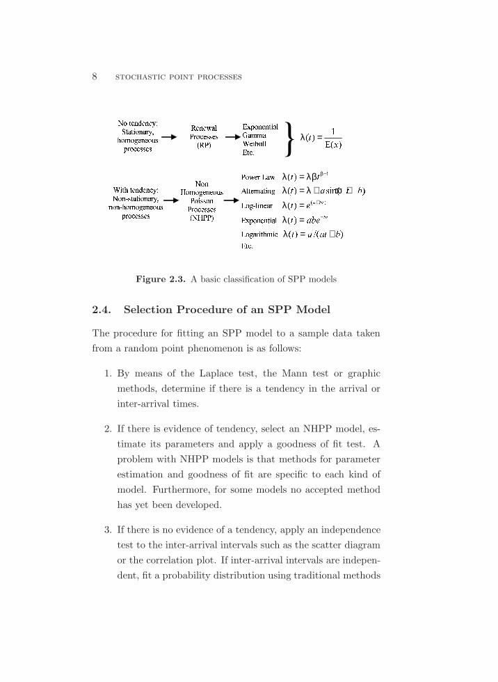
2.3. SPP Models
Figure 2.3 shows a basic classification of SPP models based on
tendency. λ, β, a, b and ω are parameters of the models.
The name for an RP is given after the x’s distribution. The
most famous RP is the exponential one, commonly called Homo-
geneous Poisson process (HPP).
For t → ∞, the intensity function of every RP is a constant
defined as the inverse of E(x), the expected value of the x’s:
λ(t) =1
E(x). (2.5)
8 stochastic point processes
�� ���������������� �������������������� ������������������� ������������������������ } ! " #! "$ %λ =���� ������������&�������� ���&�������������������� ���'����������������������������'��� ����� (� )* +, ,β−λ = λβ-��������� . / 012. /3 4 3 5λ = λ + ω +(��&����� 6 78 9 : ;<= > +λ =���������� ? @ ABC DEF−λ =(��������� G H IG HJ K KJ Lλ = +����Figure 2.3. A basic classification of SPP models
2.4. Selection Procedure of an SPP Model
The procedure for fitting an SPP model to a sample data taken
from a random point phenomenon is as follows:
1. By means of the Laplace test, the Mann test or graphic
methods, determine if there is a tendency in the arrival or
inter-arrival times.
2. If there is evidence of tendency, select an NHPP model, es-
timate its parameters and apply a goodness of fit test. A
problem with NHPP models is that methods for parameter
estimation and goodness of fit are specific to each kind of
model. Furthermore, for some models no accepted method
has yet been developed.
3. If there is no evidence of a tendency, apply an independence
test to the inter-arrival intervals such as the scatter diagram
or the correlation plot. If inter-arrival intervals are indepen-
dent, fit a probability distribution using traditional methods

the power law process 9
for parameter estimation and goodness of fit. In this case,
an RP model is obtained.
2.5. The Power Law Process
While there are many NHPP models, the approach here is to use
the Power Law Process (PLP) developed by L. Crow in 1974,
because:
• it is an accepted model to represent the failure process of
repairable components;
• there are methods for parameter estimation and goodness of
fit;
• it can represent a process with or without tendency; and
• it can represent the HPP.
The intensity function of this process is:
λ(t) = λβtβ−1 , (2.6)
where λ is the scale parameter and β the shape parameter, both
greater than zero.
The shape parameter controls the tendency of the model in
the following way:
• β > 1 for positive tendency;
• β < 1 for negative tendency; and
• β = 1 for zero tendency (in this case PLP is equal to HPP).
10 stochastic point processes
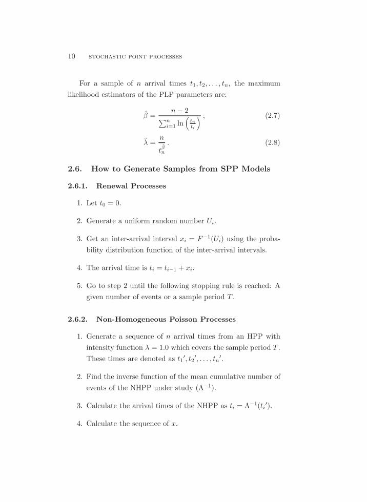
For a sample of n arrival times t1, t2, . . . , tn, the maximum
likelihood estimators of the PLP parameters are:
β =n− 2
∑ni=1 ln
(
tnti
) ; (2.7)
λ =n
tβn. (2.8)
2.6. How to Generate Samples from SPP Models
2.6.1. Renewal Processes
1. Let t0 = 0.
2. Generate a uniform random number Ui.
3. Get an inter-arrival interval xi = F−1(Ui) using the proba-
bility distribution function of the inter-arrival intervals.
4. The arrival time is ti = ti−1 + xi.
5. Go to step 2 until the following stopping rule is reached: A
given number of events or a sample period T .
2.6.2. Non-Homogeneous Poisson Processes
1. Generate a sequence of n arrival times from an HPP with
intensity function λ = 1.0 which covers the sample period T .
These times are denoted as t1′, t2
′, . . . , tn′.
2. Find the inverse function of the mean cumulative number of
events of the NHPP under study (Λ−1).
3. Calculate the arrival times of the NHPP as ti = Λ−1(ti′).
4. Calculate the sequence of x.

superposition 11
The algorithm has application if the inversion of Λ is easy. In
the case of PLP, the recursive equation is:
t =
(
t′
λ
)1/β
= Λ−1(t′) . (2.9)
2.7. Superposition
The operation of adding the events of several SPP for a given
period t is called superposition. The resulting process is a “super-
imposed process.” Figure 2.4 depicts this concept.
��� ���� � � ���� � �� ��� � � ������������� ���Figure 2.4. The superposition of several SPP
The expected number of events during t for a superimposed
SPP is the sum of the expected number of the NC SPP which
compose it:
E[N(t)]G = E[N(t)]1+E[N(t)]2+ · · ·+E[N(t)]NC =
NC∑
i=1
E[N(t)]i .
(2.10)
12 stochastic point processes
The expected number of events in an SPP is obtained from its
intensity function as:
E[N(t)] =
∫ t
0λ(t) dt . (2.11)
Replacing(2.9) into (2.8),
∫ t
0λG(t) dt =
∫ t
0λ1(t) dt+
∫ t
0λ2(t) dt+ · · ·+
∫ t
0λNC(t) dt
′ ,
(2.12)
the following relationship is obtained:
λG(t) = λ1(t) + λ2(t) + · · · + λNC(t) . (2.13)
The results expressed in (2.10) and (2.13) hold regardless of the
kind of SPP used to compose the superimposed process.

Chapter 3
Some Misconceptions About
SPP and the Modeling of
Repairable Components
Since long ago, SPP theory has been successfully applied in many
fields of knowledge such as biology, physics, queuing analysis, and
engineering reliability. Statistical procedures for applying this
type of modeling to real problems have been developed and several
SPP models have gained wide acceptance.
On the other hand, SPP has not received as much attention in
power system reliability as in other fields and only a small number
of applications have been reported. This may be due to some com-
mon misconceptions about the reliability modeling of repairable
components. In particular, it is often believed that SPP is iden-
tical to others widely used, such as the analyses based on the
Weibull distribution.
The aim of this chapter is to bring some clarity upon SPP
theory and its application in the reliability field, by discussing the
origin of these misconceptions. The content of this chapter is taken
from the paper “Some Misconceptions about the Modeling of Re-
pairable Components,” by Zapata, Torres, Kirschen and Rıos [29].
13

14 spp and the modeling of repairable components
3.1. Review of Basic Concepts
Before discussing the misconceptions, it is necessary to review
some fundamental concepts about random processes.
3.1.1. Definitions
The term random process denotes a random phenomenon that
is observed in the real world. This term is reserved for a kind of
modeling for random processes. The period of interest for studying
a random process is denoted t. A random variable x represents
the random process.
A random process is stationary if their statistical properties,
the expectation E[x] and the variance Var[x] are constant during t.
The opposite is true for a non-stationary random process.
A random process is time homogeneous if its probability den-
sity function f(x) does not change during t. The opposite is true
for a non-homogeneous random process.
Homogeneous and stationary are interchangeable terms be-
cause: (i) If f(x) does not change during t then E[x] and Var[x]
are constant during this period; and (ii) if E[x] and Var[x] are
constant during t, it is necessary that f(x) does not change dur-
ing this period. Non-homogeneous and non-stationary are also
interchangeable terms.
A distribution is a mathematical model for a stationary ran-
dom process in which t does not explicitly appear. A distribution
is defined by means of a probability density function f(x) which
does not change during t. All mathematical functions used as
distributions produce E[x] and Var[x], as this kind of model al-
ways refers to a stationary random process; hence E[x] and Var[x]
are only functions of the distribution parameters which are also
constant.

review of basic concepts 15
A stochastic process is a mathematical model for a stationary
or non-stationary random process in which t appears explicitly.
The random variable that represents the process can then be writ-
ten xt and t is called the process index. Thus, a stochastic process
is a collection of random variables xt1 , xt2 , . . . , xtN , one for each
value of the index t. Thus, there is a collection of probability
density functions ft1(x), ft2(x), . . . , ftN (x), one for each random
variable. If for a given t the statistics of the random process are
constant, it is stationary and time homogeneous because the fti(x)
do not change during this period. The opposite is true for a non-
stationary, non-homogeneous random process.
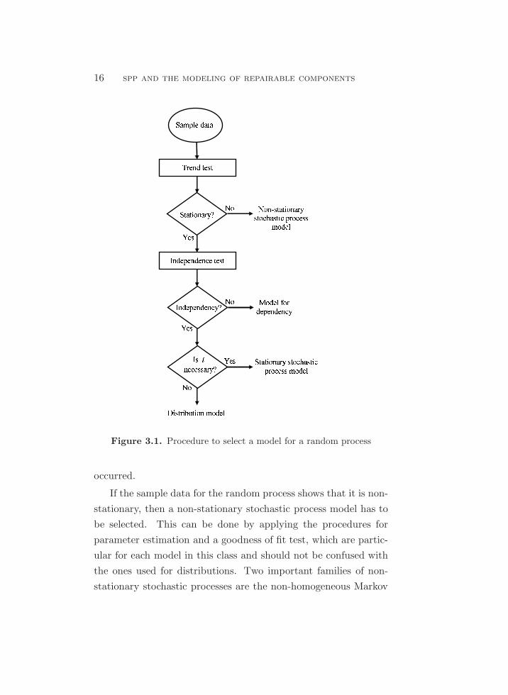
3.1.2. How to Select a Model for a Random Process
Figure 3.1 shows the basic procedure for selecting a model that is
a proper representation of a random process. Omitting any of the
three steps of this procedure can lead to an unsuitable model. A
sample x1, x2, . . . , xn is the input data for this procedure.
The first step is to determine whether the random process is
stationary or non-stationary. Several statistical methods are avail-
able for this. However, only trend tests are discussed here, because
only sequences of times to failure (ttf) and times to repair (ttr)
are considered in this chapter.
Figure 3.2 shows a simple trend test where the bar graph shows
the chronologically ordered, inter-arrival time magnitudes. If this
graph shows a pattern of increasing or decreasing inter-arrival time
magnitudes, then the random process is deemed to have a ten-
dency, or else it is non-stationary. If this test does not show that
the random process has a tendency, it is deemed to be station-
ary. The basic condition to guarantee the validity of a trend test
is to keep the chronological order in which the inter-arrival times
16 spp and the modeling of repairable components
����� �������� ��������� ��������
����������������� � ����������� ����������� �����
� ��� ����� ���� �� �������� ���� ������������� � ���� ��� � ����������� ������� ������ ������� � ���� ���
Figure 3.1. Procedure to select a model for a random process
occurred.
If the sample data for the random process shows that it is non-
stationary, then a non-stationary stochastic process model has to
be selected. This can be done by applying the procedures for
parameter estimation and a goodness of fit test, which are partic-
ular for each model in this class and should not be confused with
the ones used for distributions. Two important families of non-
stationary stochastic processes are the non-homogeneous Markov

review of basic concepts 17
�����
�������� ����� ��� ������������� ������
Figure 3.2. Bar graphs of inter-arrival times magnitudes for trend test
chains and the non-homogeneous Poisson processes.
If the sample data for the random process under study shows
it is stationary, it is necessary to apply a test for independency,
such as the scatter diagram or the correlation plot. Two cases
arise here:
1. If the sample data is not independent, a model for dependent
events has to be selected. An example of these kinds of
models is the branching point process or time series.
2. If the sample data is independent, a distribution must be
selected if t is not necessary to explain the random process.
If that is not the case, a stationary stochastic process must be
selected. In both cases it is necessary to apply the procedures
for parameter estimation and a goodness of fit test to select
the distribution or the stationary stochastic process model
that can represent the random process under study.
The importance of performing trend and independency tests
is discussed by Ascher and Hansen [2] who point out that:

18 spp and the modeling of repairable components
1. It is incorrect to fit a sample of inter-arrival times to a distri-
bution model without performing first a trend test to check
that the random process from which the sample was taken
is stationary. Goodness of fit tests sorts out sample values
by magnitude, hence losing the chronological order in which
they occurred.
2. It is incorrect to fit a sample of inter-arrival times to a distri-
bution model without performing first an independency test
because the goodness of fit tests—such as chi square and
Kolmogorov-Smirnov—were developed assuming sample in-
dependency. This also applies to the maximum likelihood
method for parameter estimation.
3.2. Reliability Analysis of Non-Repairable
Components
A non-repairable component is one that dies when the first failure
f1 occurs. The classical model for this kind of component is shown
in Figure 3.3. It only considers two operating states and ttf is used
to represent the failure process.
���������� ������ ��� � � �� ���� ����� ���������
Figure 3.3. Operating states of a non-repairable component

reliability analysis of non-reparable components 19
Because a non-repairable component can fail only once, a sam-
ple ttf1, ttf2, . . . , ttfn obtained from a group of identical compo-
nents that have failed is necessary to build its reliability model.
Figure 3.4 shows such a sample. These values are not a ordered
in a chronological sequence and each has no connection with the
other sample values. Furthermore, the instant when the observa-
tion of the operating time was taken does not matter.
�� ������ ������ �������� ����
Figure 3.4. Sample of ttf of a group of identical non-repairable com-ponents
The ttf sample is fitted to a distribution fttf (t) that is called life
model. Fttf (t) gives the probability of failure and its complement
Rttf (t) = 1− Fttf (t) is the reliability.
One important aspect to study for non-repairable components
is the risk that a component that has not failed until a given time
fails after it. This is a conditional probability that leads to the
famous equation for λ(t) called “failure rate” or “hazard rate”:
λ(t) = lim∆t→0
R(t)−R(t−∆t)
∆t · R(t)=
fttf (t)
[1− Fttf (t)]. (3.1)
Depending on the kind of distribution used for the life model or
the values of its parameters, λ(t) can be constant or a function of
time. Only for the exponential distribution λ(t) it is a constant;
20 spp and the modeling of repairable components
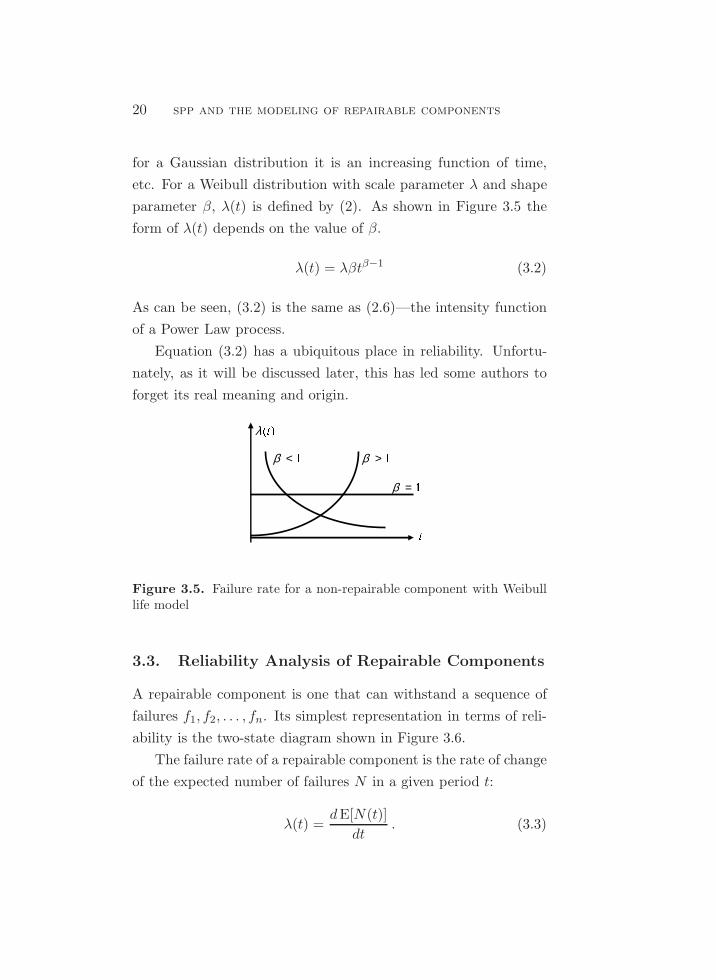
for a Gaussian distribution it is an increasing function of time,
etc. For a Weibull distribution with scale parameter λ and shape
parameter β, λ(t) is defined by (2). As shown in Figure 3.5 the
form of λ(t) depends on the value of β.
λ(t) = λβtβ−1 (3.2)
As can be seen, (3.2) is the same as (2.6)—the intensity function
of a Power Law process.
Equation (3.2) has a ubiquitous place in reliability. Unfortu-
nately, as it will be discussed later, this has led some authors to
forget its real meaning and origin.
� ��λ
� �β =
�β <
�β >
Figure 3.5. Failure rate for a non-repairable component with Weibulllife model
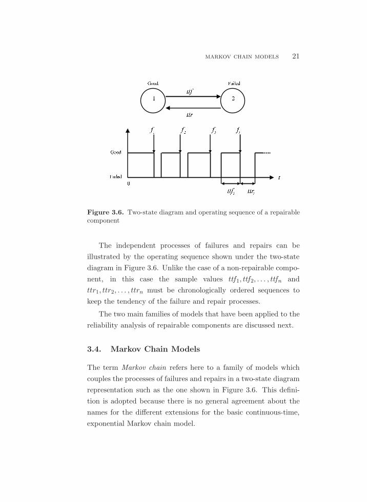
3.3. Reliability Analysis of Repairable Components
A repairable component is one that can withstand a sequence of
failures f1, f2, . . . , fn. Its simplest representation in terms of reli-
ability is the two-state diagram shown in Figure 3.6.
The failure rate of a repairable component is the rate of change
of the expected number of failures N in a given period t:
λ(t) =dE[N(t)]
dt. (3.3)
markov chain models 21
� ����� ��������
� ������������� �� �� ��
��� !""#Figure 3.6. Two-state diagram and operating sequence of a repairablecomponent
The independent processes of failures and repairs can be
illustrated by the operating sequence shown under the two-state
diagram in Figure 3.6. Unlike the case of a non-repairable compo-
nent, in this case the sample values ttf1, ttf2, . . . , ttfn and
ttr1, ttr2, . . . , ttrn must be chronologically ordered sequences to
keep the tendency of the failure and repair processes.
The two main families of models that have been applied to the
reliability analysis of repairable components are discussed next.
3.4. Markov Chain Models
The term Markov chain refers here to a family of models which
couples the processes of failures and repairs in a two-state diagram
representation such as the one shown in Figure 3.6. This defini-
tion is adopted because there is no general agreement about the
names for the different extensions for the basic continuous-time,
exponential Markov chain model.
22 spp and the modeling of repairable components
3.4.1. Homogeneous Exponential Markov Chain
If the samples of ttf and ttr show no tendency, are independent
and meet a goodness of fit test for exponential distributions with
parameters λ = 1/ ttf and µ = 1/ ttr, respectively, then the cou-
pled process of failures and repairs is described by:
dP1(t)dt
dP2(t)dt
=
−λ µ
λ −µ
P1(t)
P2(t)
. (3.4)
P1(t) and P2(t) are the probabilities of finding the component in
states 1 (good) and 2 (failed), respectively. λ and µ are called
“failure rate” and “repair rate,” respectively, or more generally
“transition rates.” Overline symbols denote a statistical mean.
The most appealing characteristic of this model is that it has an
analytical solution.
This model is memoryless or Markovian, i.e., the transition
to another state depends only on the current state and thus the
trajectory before reaching the present state does not matter. This
model is commonly called homogeneous Markov process or homo-
geneous Markov chain.
3.4.2. General Homogeneous Markov Chain
In this case, samples of ttf and ttr show no tendency, are inde-
pendent, and one or both of them meet the goodness of fit test
with a non-exponential distribution. When both distributions are
not exponential, this model is called non-Markovian process and
for the case where one is exponential but the other not it is called
semi-Markov process. We adopt the name general homogeneous
Markov chain because “general” indicates that any kind of dis-
tributions can be used and “homogeneous” specifies that these

markov chain models 23
distributions do not change over time. This model does not have
the memoryless property, i.e., it is non-Markovian and cannot be
solved using (3.4). Solution methods include the Monte Carlo sim-
ulation, the device of stages and the technique of adding variables.
This model is very important because it is unusual for both the
failure and repair distributions to be exponential. While the fail-
ure process for non-aged components generally fits an exponential
distribution, repair times are generally lognormally distributed.
3.4.3. Non-Homogeneous Markov Chain
In this case, λ and µ in (3.4) are not constant but functions of
time. The failure and repair processes are thus not homogeneous
because, as time passes, the expected number of failures and the
expected number of repairs are not constant. Therefore, the failure
and repair processes cannot be represented by means of distribu-
tions. This model also does not have the memoryless property,
i.e., it is non-Markovian. Popular solutions to this process are nu-
merical methods of differential equations and the sequential Monte
Carlo simulation. However, it has problems for adjusting the oper-
ating times, as well as of tractability of some types of time-varying
rates [6].
3.4.4. SPP Models
As shown in Figure 3.7, this kind of modeling decouples the pro-
cesses of failures and repairs of the component. Failures and re-
pairs are represented by sequences of events that arrive indepen-
dently.
In many applications the repair process is neglected because
the repair times are much shorter than the typical interval of time-
separating failures. For example, the repair time may be of the

24 spp and the modeling of repairable components
�����
������
��� ������
�������� � �� �λ������� � �� �λ
Figure 3.7. In SPP modeling the process of failures and repairs areuncoupled
order of hours, compared to times to failure in the order of years.
3.5. The Misconceptions
3.5.1. The Meaning of the Term “Failure Rate”
The first problem that arises is that the failure rate given by (3.1)
is confused with the one in (3.3) when an SPP is used to model
the failure process of a repairable component. The two concepts
are different:
1. The failure rate (3.1) refers to failures that affect a popula-
tion of identical non-repairable components and kill them.
For a single non-repairable component, it can neither be cal-
culated nor measured.
2. The failure rate (3.3) refers to failures that affect a single
repairable component if the sample was taken from a par-
ticular component. Also, it can refer to failures that affect
a population of identical or non-identical repairable compo-
nents if component failure data were pooled.
In order to distinguish the two concepts, Ascher and Fein-
gold [1] proposed the acronym ROCOF (rate of occurrence of fail-
ures) to denote (3.3). While this lexical distinction is useful, it
the misconceptions 25
is essential to understand what definition applies for repairable
and non-repairable components; it is incorrect to use the defini-
tion (3.1) for repairable components, or the definition (3.3) for
non-repairable ones. However, in many papers, (3.1) is presented
as the failure rate of components that are repairable, such as power
transformers and generators. In [15] Thompson discusses the uses
and abuses on the application of (3.1).
3.5.2. The Use of a Life Model for a Repairable
Component
The life model of a non-repairable component fttf (t) refers to the
arrival of one and only one failure that kills it. Thus, it is incor-
rect to apply this concept to a repairable component, as it can
withstand several failures. But what happens if an analyst takes
a sample of ttf from a repairable component and, after applying
required tests, shows that a given distribution is a valid repre-
sentation of this failure process and calls it the component’s life
model with failure rate defined by (1)? Although the procedure is
correct, the way the analyst conceives the model is flawed:
1. As explained before, the failure rate (3.1) does not apply.
2. The distribution represents the inter-arrival times of failures.
It can be used to calculate the probability that ttf is less or
equal than a given value, for generating a sequence of time
to failures or for defining an RP failure model with failure
rate given by (3.3).
3. The distribution is not a life model because it does not de-
fine the death of the repairable component. Such an event is
defined mainly by economic considerations: A failed compo-
nent is deemed to have died and is thus replaced if its repair

26 spp and the modeling of repairable components
cost is equal or higher than its replacement cost, or if the
expected cost of its unavailability during a planning period
is higher than its replacement cost.
3.5.3. A Distribution Can Represent a Non-Stationary
Random Process
This is the most misleading idea in reliability! A distribution can
only be used to model stationary random processes. All mathe-
matical functions used as distributions produce constant statistics.
This fact can be easily proven using a bar diagram of a sequence
of values generated from any distribution. Figure 3.8 shows this
for a realization of a Weibull distribution with λ = 5 [years] and
different values of β. As it can be seen there is no tendency in any
case.
Similarly, RP are always stationary because they are defined on
the basis of the distribution of inter-arrival times. Thus, Thomp-
son [15] points out that an RP cannot model component aging and
discusses this misconception.
This misconception originates from (3.1); as it can produce
increasing or decreasing failure rates depending on the kind of
distribution or in accordance with the value of its shape param-
eter, it is believed (or, more precisely, misbelieved) that this is
a natural property of some distributions. Thus, in some papers
a time-varying failure rate is defined for a repairable component
and, without a theoretical support, the ttf are generated using an
exponential or Weibull distribution.

the misconceptions 27
Figure 3.8. Bar graphs of the values generated from a Weibull distri-bution
3.5.4. Equation (3.2) Generates a Random Process Whose
Model is the Weibull Distribution
This misconception is a consequence of the previous one. The
truth is that, if (3.2) is used as an intensity function for an SPP
or as a transition rate for a Markov chain, then an HPP is ob-
tained when β = 1, and a non-stationary one when β 6= 1. This
can be proven using the algorithm given in section 2.6.2. More
importantly, this is valid for any random process and not only
for those which pertain to failures. The relationship between the
Weibull distribution and (3.2) is restricted only to the case where
the reliability of a non-repairable component is studied.
28 spp and the modeling of repairable components
This misconception originates from the fact that the concept
expressed by (3.2) has been applied extensively in the reliability
field, forgetting in many cases its origin and meaning. For exam-
ple:
1. Many books and papers show it as a natural property of the
Weibull distribution. Results obtained by means of (3.2) are
only valid when referring to the reliability of a non-repairable
component, a particular result of an application where the
Weibull distribution is applied.
2. Many papers define the failure rate for a repairable compo-
nent using (3.2) and assert that it belongs to the Weibull
distribution, although they are applying a proper method
for a non-stationary analysis. That is, the analysis is correct
but they are bringing a concept that does not apply.
3.5.5. A General Homogeneous Markov Chain Can
Represent a Non-Stationary Process
This misconception is also a consequence of the third misconcep-
tion. It is not true because a distribution always refers to a sta-
tionary process. The bar diagram shown in Figure 3.8 proves this
for a Weibull distribution. In addition, let us consider now the
method called the device of stages, viz., for some pairs of distribu-
tions (exponential-lognormal, exponential-Weibull, etc.), it trans-
forms the two-state general homogeneous Markov chain in an ex-
ponential one that has more than two states. Figure 3.9 shows an
example: The exponential-lognormal chain is transformed into an
exponential one where state 2 is replaced by k stages in series (2S1
to 2Sk) and two stages in parallel (SP1 and 2P2).
Transition rates ρ, ρω1, ρω2, ρ1, and ρ2 are constants obtained
from the four first moments of the lognormal distribution. If the

the misconceptions 29
� ����� ����� � � �� � ������������ � ���� ! "�#��$%��� �&'�('�()
λ �&*����ρ ρ+ρω,ρω
�����-ρ.ρ
Figure 3.9. The device of stages for solving a given homogeneousMarkov chain
equivalent exponential Markov chain obtained using the device of
stages, which is stationary, solves the two-state general homoge-
neous Markov chain, how can the latter be non-stationary? How-
ever, some papers apply the device of stages and say that for the
case Weibull-lognormal it represents a non-stationary process!
This misconception originates from incorrectly believing that
the transition rates of a general homogeneous Markov chain are
defined by means of (3.1). This is wrong because there is no con-
nection between the concepts of transition rate of a Markov chain
and hazard rate of a non-repairable component. Concept (3.1)
cannot be extended to failures of a repairable component nor to
other events such as repairs.

30 spp and the modeling of repairable components
3.5.6. The PLP is the Same Thing as a Weibull
Distribution
The arguments presented in section 3.5.4 show that this is false.
The PLP has no connection with the Weibull distribution. The
origin of this misconception is the fact that the PLP intensity
function is the mathematical function (3.2). However, when ap-
plying (3.2) the context of application should be remembered:
1. For a non-repairable component, it refers to a sequence of
failures that affect a population of identical non-repairable
components, not to the process of failure arrivals to a single
non-repairable component nor to the arrival of other, non-
failure events.
2. For a repairable component, it refers to a sequence of events
that arrive. It is not confined to the case of failures. And
in the case of failures, it can represent the process of fail-
ure arrival to a repairable component or to a population of
repairable components.
3.5.7. The PLP is the Same Thing as a Weibull RP
The arguments presented in section 3.5.5 can be used to show
that this is a misconception. In a PLP an exponential stationary
process is obtained when β = 1 and a non-stationary one when
β 6= 1. When β = 1 it generates a HPP, not a Weibull RP.
This misconception has the same origin that the one discussed in
section 3.5.6.
Another factor that reinforces this misconception is that PLP
has received other names with the word Weibull such as Weibull
process, Weibull-Poisson process, Rasch-Weibull process [9].

relationship between spp and markov chains 31
3.5.8. The Only Model for a Stationary Failure Process
is the HPP
This is probably the most common of all misconceptions, but it is
not as misleading as the one discussed in 3.5.4.
This statement is only valid when a sample of ttf taken from
repairable component shows no tendency, is independent and com-
plies with the goodness of fit test for an exponential distribution.
But what happens if the sample shows no tendency, is indepen-
dent, but does not comply with a goodness of fit test for the ex-
ponential distribution? In this case, it is incorrect to assume an
exponential distribution; the failure process of the repairable com-
ponent has to be represented by means of the RP of a distribution
that satisfies a goodness of fit test.
This misconception originates again from the concept of failure
rate for a non-repairable component (3.1); it produces a constant
failure rate only for the case of an exponential distribution. Thus,
“constant failure rate = HPP model” has been applied as a rule of
thumb for any type of components, forgetting that this result was
obtained only for non-repairable ones. For the case of a repairable
component with stationary failure process, all RP are possible
failure models.
3.6. Relationship Between SPP and Markov Chains
A two-state Markov chain is generated by two SPP processes, as
shown in Figure 3.10. Every time a failure arrives to the compo-
nent, it is sent from the good state to the failed one; and every
time a repair is performed, the component comes back to the good
state. The sources of this motion are the SPP.
Intensity functions λF (t) and λR(t) in the SPP models are
equal to transition rates λ12(t) and λ21(t) in the Markov chain,

32 spp and the modeling of repairable components
�����
������
��� ������
��������� � �� �λ
�������� � �� λ
Figure 3.10. Relationship between a two-state Markov chain and SPP
respectively, regardless of whether the models are defined using
distributions or non-stationary stochastic processes.
One could therefore argue that, since both types of models are
equivalent, there is no reason to use an SPP when Markov chains
are a more popular method. While this would be true at the com-
ponent level, analysts usually deal with systems of repairable com-
ponents. When dealing with large repairable systems, the repair
process should not be included in the component level because:
1. It is equivalent to assume repair resources are unlimited be-
cause every time the component fails a crew is available to
repair it, or in other words, there is a repair team dedicated
to each component. Hence, an implicit assumption is made
that repair times depend only on the particular actions taken
to fix each type of component.
2. For maintenance purposes, a power system is usually split
into several zones or service territories, and repair teams are
assigned to each area. The repair process performed in each
service territory is really a queuing system.
SPP modeling thus makes it possible to represent the repair
process performed in each area of a large repairable system as it

conclusions 33
really happens. This is something that Markov chain modeling is
unable to do.
3.7. Conclusions
There are several common misconceptions about the modeling of
repairable components for reliability studies. In particular, it is
often assumed that SPP are identical to other methods currently
in widespread use, for example, the popular analyses based on the
Weibull distribution.
All these misconceptions originate in the incorrect practice of
analyzing the reliability of repairable components using concepts
that were developed only for non-repairable ones and, specifically,
in the misleading idea that a stationary random process model can
represent a non-stationary random process.
Reliability engineers must consider carefully the concepts of
homogeneity and stationarity of random processes, the procedure
for selecting a type of model for a random process, and the differ-
ences between the main types of models that are available.

Chapter 4
The Repair Process in a
Power System
The aim of this chapter is to show why the repair process per-
formed in a power system should not be modeled as part of the
component reliability models but independently using queuing the-
ory concepts. This also justifies the use of SPP as a modeling
method for reliability assessments. In order to deepen this sub-
ject, data of the repair process performed in three Colombian dis-
tribution systems was used to apply the proposed approach of
modeling.
The content of this chapter is taken from the paper “Modeling
the Repair Process of a Power Distribution System,” by Zapata,
Silva, Gonzalez, Burbano and Hernandez [26].
4.1. Introduction
For maintenance purposes the power distribution system is split
into several zones or service territories, each one assigned to a
repair team, as shown in Figure 4.1.
The resources for repairs are the personnel, trucks, tools, spares,
etc. available for this work. The way these resources are organized,
35

36 the repair process in a power system
������ ����������
� ��������� ����� �����Figure 4.1. Zones for maintenance in a power distribution system
for example, the number of crews for each zone, is the logistics.
The repair resources generate the repair process.
The repair process is the sequence of repairs performed by
crews in accordance with the repair orders sent by the control
center, which either automatically detects component failures or
receives customer calls regarding service interruptions. Thus, the
repair process in each service territory is a queuing system. The
input to this system is the sequence of component failures which
produce service interruptions that have to be repaired by crews.
The output of this system is the sequence of service restorations
performed by crews.
The performance of the repair process is dependent on the
quality and quantity of repair resources and the logistics. These
resources are limited and have to be carefully matched to follow
the pace of component failures in order to obtain acceptable outage
times.
Another important thing to point out is that traditional re-
liability assessment of power systems has usually not considered
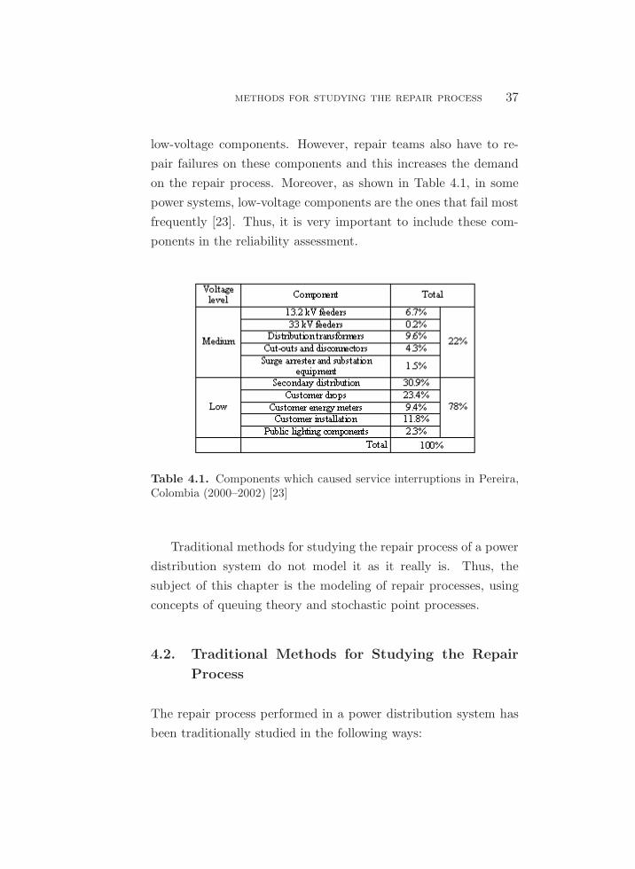
methods for studying the repair process 37
low-voltage components. However, repair teams also have to re-
pair failures on these components and this increases the demand
on the repair process. Moreover, as shown in Table 4.1, in some
power systems, low-voltage components are the ones that fail most
frequently [23]. Thus, it is very important to include these com-
ponents in the reliability assessment.
Table 4.1. Components which caused service interruptions in Pereira,Colombia (2000–2002) [23]
Traditional methods for studying the repair process of a power
distribution system do not model it as it really is. Thus, the
subject of this chapter is the modeling of repair processes, using
concepts of queuing theory and stochastic point processes.
4.2. Traditional Methods for Studying the Repair
Process
The repair process performed in a power distribution system has
been traditionally studied in the following ways:

38 the repair process in a power system
4.2.1. By Means of Statistical Analysis of Outage Times
These kinds of studies take operating data of the power distribu-
tion system and analyze the statistics of outage times by feeders,
substations and geographical zones to give guidelines about which
zones of the system need improvement on the repair process per-
formance.
Although these kinds of studies can include the modeling of
the outages times using probability distributions or stochastic pro-
cesses, they do not include an explicit modeling of the repair pro-
cess.
As a service territory can include parts of several feeders, these
kinds of studies have to be extended to each service territory be-
cause, in this case, a global analysis can be misleading.
4.2.2. As Part of the Component Reliability Models
This approach is extensively applied in power distribution relia-
bility assessments no matter the methodology (cut-sets, analytical
simulation, the Markov process or the Monte Carlo simulation):
the repair process is included as part of component reliability mod-
els, by means of the probability distribution of times to repair.
This approach has the following disadvantages:
• No matter the probability distribution used, it is assumed
repair resources are unlimited because every time a compo-
nent fails a crew is available to repair it. Hence, the repair
time only depends on the particular actions taken to fix each
kind of component.
• As the repair process is represented by means of a proba-
bility distribution, it is assumed it is a stationary process,
i.e., the performance of repair teams is not affected by in-
modeling of the repair process 39
ternal or external factors. However, in real life, the crew
performance is affected by external factors—weather, traffic,
etc.—and also by internal factors—available tools, available
skills, workload, etc.
• The tendency of the repair process performed in the power
distribution system is lost because the times to repair are
classified by component type and thus the chronological se-
quence in which they occur is lost.
• Most methods apply the n − 1 loss of component criteria.
That is not a true assumption because a failure can occur
independently, if other failures which occurred before have
been repaired or not.
• Reliability assessments of power distribution systems only
include high-voltage and medium voltage components. In
real life, however, repair teams also have to repair the low-
voltage components, a fact that causes an important demand
on repair resources. Moreover, reliability surveys shows that
in some power distribution systems the low-voltage compo-
nents are the ones that fail more frequently.
4.3. Modeling of the Repair Process
The repair process of each zone (service territory) of a power dis-
tribution system is modeled as the queuing system shown in Fig-
ure 4.2.
For this queuing system the following is defined:
• Clients: Failures which produce service interruptions and
have to be repaired by crews.
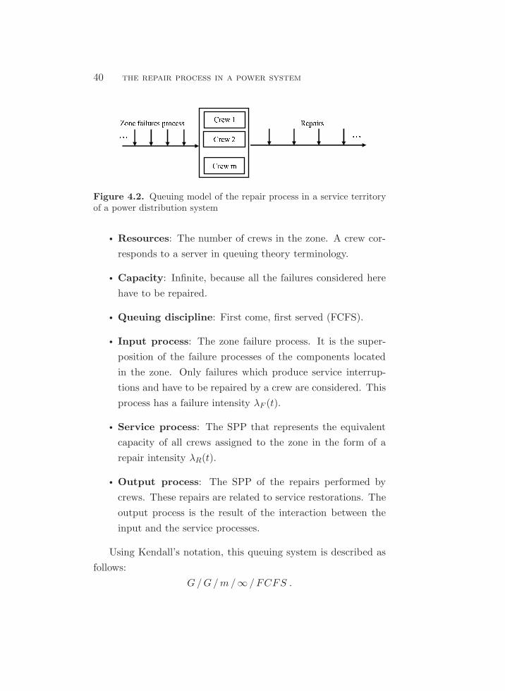
40 the repair process in a power system
����� ������ �� ��� ���������� ���� ���� �Figure 4.2. Queuing model of the repair process in a service territoryof a power distribution system
• Resources: The number of crews in the zone. A crew cor-
responds to a server in queuing theory terminology.
• Capacity: Infinite, because all the failures considered here
have to be repaired.
• Queuing discipline: First come, first served (FCFS).
• Input process: The zone failure process. It is the super-
position of the failure processes of the components located
in the zone. Only failures which produce service interrup-
tions and have to be repaired by a crew are considered. This
process has a failure intensity λF (t).
• Service process: The SPP that represents the equivalent
capacity of all crews assigned to the zone in the form of a
repair intensity λR(t).
• Output process: The SPP of the repairs performed by
crews. These repairs are related to service restorations. The
output process is the result of the interaction between the
input and the service processes.
Using Kendall’s notation, this queuing system is described as
follows:
G/G/m/∞ /FCFS .
assessment of the repair process performance 41
The first and second G indicate that both the input and service
processes are general SPP (RP or NHPP). m, ∞, and FCFS
indicate, respectively, the number of crews, the system capacity
and the queuing discipline.
The traffic intensity index a(t) is defined as:
a(t) =λF (t)
λR(t). (4.1)
Although a(t) is dimensionless, it is measured in Erlangs. A traffic
intensity of 1.0Erlang means one failure uses or occupies the repair
resources 100% of the time. Traffic intensity higher than 1.0 means
the failures arrive faster than repairs can be performed. Thus, a(t)
have to be less or equal to 1.0 in order to have a stable queuing
system.
4.4. Assessment of the Repair Process Performance
4.4.1. Obtaining the Zone Failure Process
From operating records, obtain a sample of arrival times of those
component failures which caused service interruptions and were
repaired by crews. It is recommended the sample covers at least
one year of system operation.
It is important to remember that:
• Not all service interruptions are solved by crews; some of
them are solved by means of a reconnection performed by a
circuit breaker or recloser.
• Low-voltage components also cause service interruptions which
in most of the cases have to be repaired by crews.
Apply to the failure arrival-times sample the procedure for
selecting an SPP model. In accordance with the tendency on the
resulting zone failure process, the following can be concluded:
42 the repair process in a power system
• Zero tendency: The population of components located in
the zone is in its useful life. That is, their reliability is neither
improving nor deteriorating.
• Positive tendency: The population of components located
in the zone shows aging.
• Negative tendency: The population of components lo-
cated in the zone shows reliability improvement.
This kind of modeling implies repairs are minimal, i.e., they
only return the components to the operating state without im-
proving or deteriorating their reliability condition.
4.4.2. Obtaining the Zone Service Process
For each failure that caused a service interruption and was repaired
by means of a crew action, obtain the time to repair (ttr).
Time to repair includes: transportation time to the place where
customers are without service, time to find the failed component,
time to fix the failed component and reconnection time.
A ttr does not include the waiting time (tw) the period during
which the crew receives the repair order and is free to go to repair
the failure. The waiting time is a result of the congestion on the
repair process, i.e., the fact that when a crew receives a repair
order, it can be busy repairing a failure that occurred before.
Apply to the sample of times to repair the procedure for se-
lecting an SPP model. In accordance with the tendency on the
resulting service process the following can be concluded:
• Zero tendency: The crew performance is neither increasing
nor decreasing.
• Positive tendency: The crew performance is increasing be-
cause, as time passes, repairs takes less time to be performed.
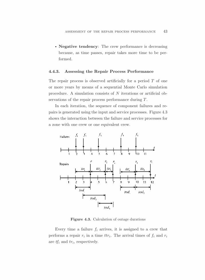
assessment of the repair process performance 43
• Negative tendency: The crew performance is decreasing
because, as time passes, repair takes more time to be per-
formed.
4.4.3. Assessing the Repair Process Performance
The repair process is observed artificially for a period T of one
or more years by means of a sequential Monte Carlo simulation
procedure. A simulation consists of N iterations or artificial ob-
servations of the repair process performance during T .
In each iteration, the sequence of component failures and re-
pairs is generated using the input and service processes. Figure 4.3
shows the interaction between the failure and service processes for
a zone with one crew or one equivalent crew.
��������� � � � � � �� ���� �� �� �� �� �� � � � � ! " # �$ �� ��%& '( )* +, -(
./01 23456�7���� �899: ;<<= >??& @AABCDDE
F345 GHIJ KLMNFigure 4.3. Calculation of outage durations
Every time a failure fi arrives, it is assigned to a crew that
performs a repair ri in a time ttri. The arrival times of fi and ri
are tfi and tri, respectively.

44 the repair process in a power system
Each iteration produces a sample of number of failures (nf),
times to repair (ttr), outage duration (tod) and waiting times (tw).
Two stopping rules may be used for the simulation: a fixed
number of iterations, or the coefficient of variation of a load point
index.
4.4.4. Iteration Procedure
1. Generate the input process for a period T using the zone
failure SPP model.
2. Generate the service process. That is, for each failure fi
generate a ttri using the zone service SPP model.
3. Compute the mean traffic intensity ma(t).
4. The arrival time of the first repair is:
tr1 = tf1 + ttr1 . (4.2)
5. The arrival time of the next repair is determined in the fol-
lowing way:
• Congestion: If all crews are busy when failure arrives,
this failure has to wait until some crew finishes a repair j
and fixes it:
tri = trj + ttri . (4.3)
• No congestion: If a crew is free when failure arrives, the
repair for this failure starts immediately.
tri = tfi + ttri . (4.4)
examples 45
6. Calculate the outage duration:
todi = tri − tfi . (4.5)
7. Calculate the repair waiting time:
twi = todi − ttri . (4.6)
8. For T or its sub-periods (month, semester, etc.) compute the
mean waiting time (mtw), the mean outage duration (mtod)
and the congestion (C) defined as:
C =mtw
mtod· 100% . (4.7)
4.5. Examples
Traditional queuing analyses assume the input and service pro-
cesses are Markovian (both HPP) or semi-Markovian (one HPP
and the other an RP). However, for the repair process of a power
distribution systems it is not known which SPP models can rep-
resent this processes.
Thus, data of three Colombian power distribution systems was
gathered in order to know these models and to apply the proposed
methodology. Table 4.2 shows general description of the studied
systems.
For each system an assessment of the repair process perfor-
mance was carried out for T = 1.0 year with simulations of 150
iterations. Tables 4.3 to 4.8 show the results. Confidence level of
input and service process models is 95%.
These results show the following:
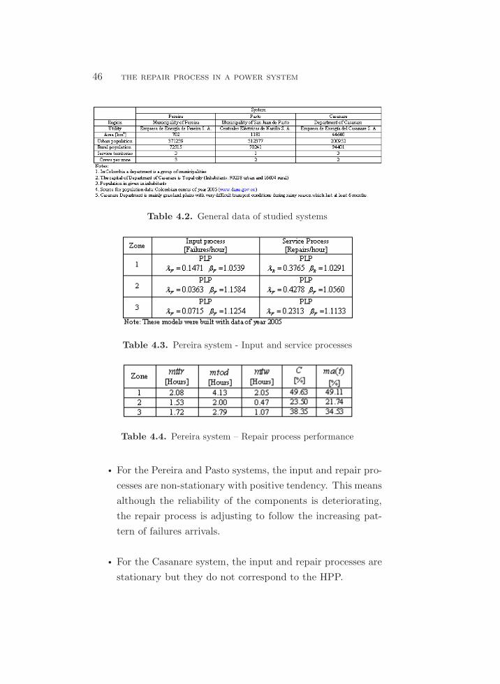
46 the repair process in a power system
Table 4.2. General data of studied systems
Table 4.3. Pereira system - Input and service processes
Table 4.4. Pereira system – Repair process performance
• For the Pereira and Pasto systems, the input and repair pro-
cesses are non-stationary with positive tendency. This means
although the reliability of the components is deteriorating,
the repair process is adjusting to follow the increasing pat-
tern of failures arrivals.
• For the Casanare system, the input and repair processes are
stationary but they do not correspond to the HPP.
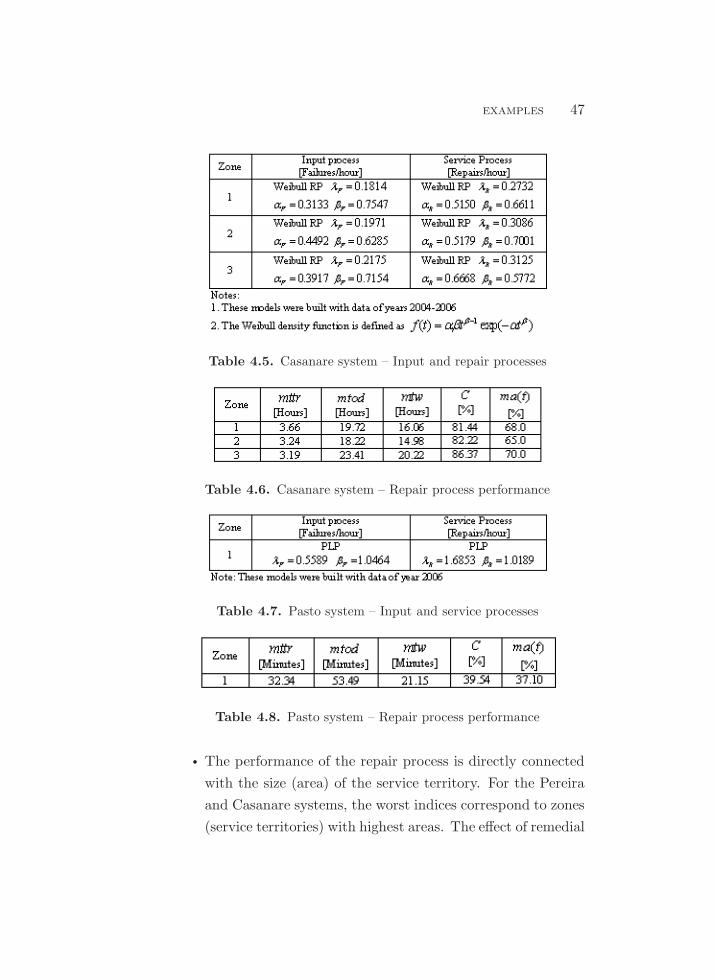
examples 47
Table 4.5. Casanare system – Input and repair processes
Table 4.6. Casanare system – Repair process performance
Table 4.7. Pasto system – Input and service processes
Table 4.8. Pasto system – Repair process performance
• The performance of the repair process is directly connected
with the size (area) of the service territory. For the Pereira
and Casanare systems, the worst indices correspond to zones
(service territories) with highest areas. The effect of remedial

48 the repair process in a power system
actions proposed to reduce outage durations can be tested
with this methodology.
• A low congestion or traffic intensity does not mean a low
waiting time or consequently a low outage duration.
• The results of mean outage time correspond to those values
observed during operation of the studied systems.
4.6. Conclusions
The repair process performed in each service territory of a power
distribution system is a queuing system. Thus, it has to be mod-
eled using queuing models, not as part of component reliabil-
ity models—the traditional approach applied in reliability assess-
ments. Also, it is not realistic to apply the deterministic criteria
n− 1 for reliability assessments of this kind of system, as a failure
can occur independently if the previous failure has been or not
repaired.
As shown in the examples, the input and service of the repair
process of a power distribution system are not necessarily HPP;
they can be RP or NHPP, and for this reason, the system reli-
ability assessment has to be performed by means of a sequential
Monte Carlo simulation. The approach presented here, which con-
siders stationary and non-stationary SPP for the failure and the
service processes, is very different from traditional queuing mod-
eling that assumes that these processes are Markovian (HPP) or
semi-Markovian (one HPP and the other an RP).
The index better reflecting the performance of the repair pro-
cess is the waiting time. A low congestion or traffic intensity does
not necessarily mean a low waiting time or consequently a low out-
age duration. The proposed methodology explicitly evaluates the

conclusions 49
performance of the repair process performed in a power distribu-
tion system and gives an analytical base for the optimal scheduling
of the repair resources, in accordance with the failure process gen-
erated by the components and the targets for reliability indices.


Chapter 5
Reliability Assessment of a
Power Distribution System
The aim of this chapter is to show how the methodology of reli-
ability assessment of a power system using SPP modeling and a
sequential Monte Carlo simulation works. This is the first stage of
development of a more comprehensive method that will be applied
to assess the vulnerability of a composite system.
5.1. Introduction
Although methods to take aging and limited resources into account
have been developed in the general reliability field and in queuing
theory, these methods are not currently in widespread use in power
distribution reliability assessment.
With regard to aging, published studies can be categorized as
follows:
1. Studies at the component level: Aging is studied for given
populations of components. This is the category with the
most publications. Studies in this category can be subcate-
gorized into:
51

52 reliability assessment of a power distribution system
• Those which model aging and external events that increase
the failure rate.
• Those which link reliability and maintenance, and deter-
mine an optimal preventive maintenance strategy to im-
prove the components’ reliability. The limitation of this
type of studies is that they do not directly connect the
components’ reliability condition to customer reliability in-
dices.
2. Studies at the system level: few papers have been written
on the effect of component aging on load point reliability
indices.
Regarding the repair process performed in power systems, it
has been traditionally included in the reliability model of the com-
ponents. This implies that repair resources are assumed unlimited,
which is unrealistic.
5.2. Traditional Component Modeling
Figure 5.1 shows the basic and most popular reliability model for
repairable components. This model is defined by the probability
distributions of time to failure (ttf) and time to repair (ttr).
�����
������
���
Figure 5.1. Two-state component reliability model
A probability distribution model always refers to a station-
ary process; hence, it always produces constant statistics (mean,
variance). This means that, no matter what kind of distribution is
traditional component modeling 53
used for the reliability model, the expected number of failures that
occur and the expected number of repairs that can be performed
do not change as time passes. In other words, failure and repair
intensities remain constant.
This kind of modeling has the following limitations:
1. Aging is not considered: Constant failure intensity means
the component reliability does not improve or deteriorate,
i.e., it is in its useful life period. This also means the com-
ponent is under “renewal” because every time it fails, it is
returned to an “as new” state. For this reason, this model
is also known as an “alternating renewal process.”
2. Repair resources are unlimited: As the repair process is in-
cluded in the component model, it is assumed that every
time the component fails a crew is available to repair it;
hence, repair time only depends on the particular actions
taken to fix each type of component. Constant repair inten-
sity means the performance of repair teams is not affected
by internal or external factors. However, in real life, a crew
has to fix all failed components located in its service terri-
tory. This means that some of them may have to wait while
the ones that failed before are repaired. Also, crew perfor-
mance is affected by external factors, such as weather and
traffic, and also by internal factors, such as available tools
and skills.
These limitations are also present in models with more than
two states and in the simplified modeling that represents a re-
pairable component as a block defined by means of a constant
failure rate (λ) and a mean repair time (r).
54 reliability assessment of a power distribution system
5.3. Methods in Widespread Use for Reliability
Assessment of Distribution Networks
5.3.1. The Homogeneous Markov Process
If the failure and repair models of every component are exponen-
tial, the system model is a homogeneous Markov process. The
mathematical model of a system with n components is the set of
ordinary differential equations:
[P ]t = [M ]t[P ]t , (5.1)
where [P ] is a row vector with the probabilities of the n ∗ n states
and [M ] is the stochastic matrix of transition intensities between
states.
Although this approach is very appealing because it gives an-
alytical solutions, it has the following disadvantages:
1. For systems with many components, such as distribution
networks, there is a huge number of system states. This
makes its application a cumbersome task.
2. Repair times of power distribution components are, in gen-
eral, log-normally distributed.
3. Loads are considered constant.
This method can include common mode outages and loss of
component criteria of any order. However, some applications re-
strict its application to the n− 1 case.
5.3.2. Device of Stages
If the distribution of the failure process or of the repair process
(or of both) is not exponential, the previous method does not
reliability assessment of distribution networks 55
apply. For some pairs of distributions (exponential-lognormal,
exponential-Weibull), this model can be transformed into a homo-
geneous Markov model by means of the device of stages method.
Although this method solves the problem of non-exponentially dis-
tributed repair times, the resulting component model has more
than two states, a fact that increases the dimension of the set of
system equations. Thus, the first and third disadvantages of the
previous method also hold for this one.
5.3.3. Simplified Method of Blocks
In this method, the system is represented as a network of compo-
nents which are connected in series or parallel. It is also known as
“minimal cut set method.” Each component is represented by a
block with a constant failure rate (λ) and a constant mean repair
time (r). A sequential reduction of series and parallel components
can be used to solve the network of blocks.
As this method is derived from the homogeneous Markov pro-
cess, it inherits disadvantages 2 and 3 of that method and adds
the following:
1. It only gives expected values of the load point indices of
failure frequency, mean time to repair and unavailability.
2. It does not consider the loss of more than one component.
5.3.4. Analytical Simulation
This method is an extension to the simplified method of blocks.
It determines the fault contribution of each component and their
impact on load points by means of the enumeration of each possi-
ble system state. In this method, each component is represented
by the same parameters used in the simplified method of blocks.

56 reliability assessment of a power distribution system
Although this method can handle the loss of more than one com-
ponent, it retains disadvantages 1, 2 and 3 of the Markov method
and disadvantage 1 of the simplified method of blocks.
5.3.5. The Monte Carlo Simulation
This method can include any kind of distributions, time-varying
loads, unbalanced conditions, common mode outages, etc. Disad-
vantages of this method are:
1. The high computational time required.
2. Multiple analyses on the same system could produce slightly
different results.
3. It can overlook rare but important system states because it
is not an enumerative method.
Disadvantages 1 and 3 can be mitigated by applying variance
reduction techniques or importance sampling.
Although this method can include loss of component criteria
of any order, it is often restricted to then− 1 case.
5.4. Methods for System Reliability Assessment that
Can Include Aging
5.4.1. Manual Approach
In the methods listed in the previous section, component failure
intensities are manually changed, for example, from their current
values to the ones they are expected to have in the future or under
a scenario where a given preventive maintenance strategy is ap-
plied. Scenarios for improvement and deterioration of the repair
intensities can also be included.

methods that can include aging 57
5.4.2. The Non-Homogeneous Markov Process
This method can include improvement and deterioration in the
failure and repair processes. However, because the repair process is
included in the reliability model of the component, the assumption
is still made that unlimited repair resources are available. This
model has disadvantages 1 and 3 mentioned for the homogeneous
one. Solutions to this kind of process are numerical. However,
this method has problems adjusting the operating times and of
tractability of some types of time-varying rates [6].
5.4.3. Stochastic Point Processes
In the general reliability field, the modeling of the failure process of
repairable components by means of SPP started in the 1960s. The
procedures for applying this kind of modeling are now well estab-
lished and applications are mainly focused on reliability analysis
of component populations.
In the power systems field, before the year 2000, applications
focused on the reliability of component populations. For example,
Schilling et al. studied thermal generators [12], Kogan and Jones
studied underground cables [11], and Kogan and Gursky studied
transmission towers [10].
In 2000, Stillman [13] applied this kind of modeling to the
reliability of a distribution network considering it as a whole entity
and showed results for rural and urban systems. He extended the
method to distribution feeders, but again treating them as a whole
entity [14]. In 2004 Balijepalli, Venkara and Christie [3] used this
kind of modeling to obtain the distributions of load point indices
of a real system. They used RP models for failures and repairs.
Failure models were obtained from data but repair models were
assumed.

58 reliability assessment of a power distribution system
5.5. Proposed Methodology
5.5.1. Modeling of Component Failure Processes
Component failures and common mode failures are modeled as
independent failure sources using PLP or RP. When a PLP model
is used:
• if β > 1 the component is aging;
• if β = 1 the component is in its useful life or as new; and
• if β < 1 the component reliability is improving.
This kind of modeling implies that repairs are minimal, i.e.,
they only return the component to the operating state without
improving or deteriorating its reliability condition.
If a component has two or more operating states, its failure
process is represented by an SPP for each one. For example, a
power transformer with operating states 100MVA (ONAF) and
80MVA (ONAN) requires two SPP failure models.
To obtain a component failure model, a sample of arrival or
inter-arrival failure times is needed. This process includes failures
caused by aging and other external factors like weather. A com-
mon approach in distribution networks is to pool data by com-
ponent class in order to obtain one model that represents each
component in a class. When using NHPP all failure models have
to be synchronized to the same time reference.
5.5.2. Modeling of Repair Process
The repair process performed in each service territory of the distri-
bution network is modeled by the queuing. This kind of modeling
is explained in Chapter 4.

system reliability assessment 59
5.6. System Reliability Assessment
System operation is observed artificially for a period T of one
or more years of interest by means of a sequential Monte Carlo
simulation algorithm. As Figure 5.2 shows, a simulation consists
of N iterations or artificial observations of system performance
under a scenario defined by topology, expansion/upgrading, and
forecasted demand.
*
*
� � ����� � �� �� � ��� � ��� ��
�� �� ���� ��* * *
������ !"�Figure 5.2. Simulation procedure
The sequence of component failures and repairs is generated
for each iteration; this is depicted in Figure 5.2 by an asterisk (∗)
that indicates when a component fails and is repaired.
For a load point K, the samples of output variables such as
the number of failures (nfk) and the down time (tdk) allow the
computation of reliability indices. Two stopping rules may be used

60 reliability assessment of a power distribution system
for the simulation: a fixed number of iterations, or the coefficient
of variation of a load point index.
5.6.1. Iteration Procedure
1. Generate the failure processes of the components and the
common mode failure processes for T .
2. Determine for each zone the failure process which consists of
the superposition of the failure processes of all components
located in the zone, including the common mode failures.
3. Generate a repair process. That is, for each failure fi gener-
ate a ttri.
The arrival time of the first repair is:
tr1 = tf1 + ttr1 . (5.2)
The arrival time of the next repair is determined in the fol-
lowing way:
• Congestion: If all crews are busy when failure i arrives,
this failure has to wait until some crew finishes a repair j
and fixes it.
tri = trj + ttri . (5.3)
• No congestion: If a crew is free when failure i arrives,
the repair for this failure starts immediately:
tri = tfi + ttri . (5.4)
4. Calculate the outage duration:
todi = tri − tfi . (5.5)
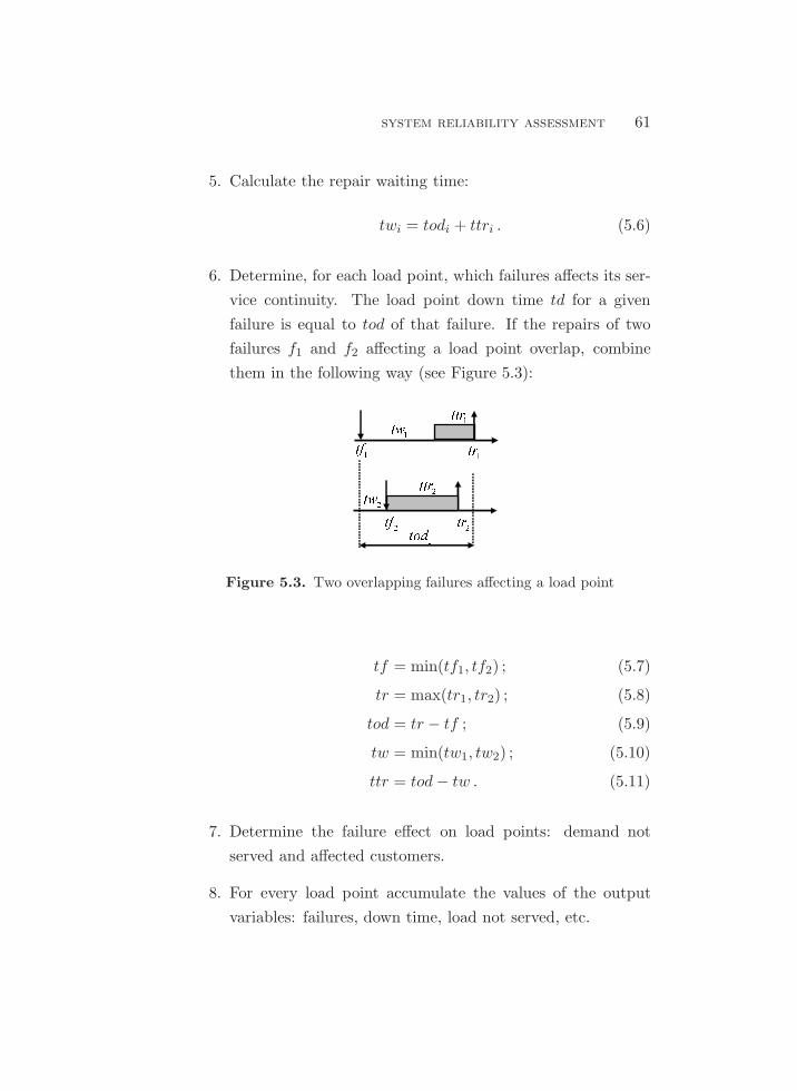
system reliability assessment 61
5. Calculate the repair waiting time:
twi = todi + ttri . (5.6)
6. Determine, for each load point, which failures affects its ser-
vice continuity. The load point down time td for a given
failure is equal to tod of that failure. If the repairs of two
failures f1 and f2 affecting a load point overlap, combine
them in the following way (see Figure 5.3):
��� ���
��� � ��� �� ��� ��� ����
Figure 5.3. Two overlapping failures affecting a load point
tf = min(tf1, tf2) ; (5.7)
tr = max(tr1, tr2) ; (5.8)
tod = tr − tf ; (5.9)
tw = min(tw1, tw2) ; (5.10)
ttr = tod− tw . (5.11)
7. Determine the failure effect on load points: demand not
served and affected customers.
8. For every load point accumulate the values of the output
variables: failures, down time, load not served, etc.

62 reliability assessment of a power distribution system
5.6.2. Repair Process Indices
For each zone and sub-period of T (month, semester, etc.) com-
pute the mean waiting time (mtw), the mean outage duration
(mtod) and the congestion (C) defined as:
C =mtw
mtod· 100% . (5.12)
5.6.3. Load Point Indices
For each load point k and sub-period of T (month, semester, etc.)
compute the adequacy indices. For example:
• Expected failure frequency:
λk =N∑
i
nfki
N. (5.13)
• Mean time to repair:
rk =
∑Ni=1 tdki
∑Ni nfki
. (5.14)
5.7. Example
Consider the overhead rural distribution system shown in Fig-
ure 5.4. For maintenance purposes, this system is split into two
zones, each assigned to a crew.
Table 5.1 shows the components’ reliability data. Most of this
data is taken from surveys performed in a Colombian system dur-
ing the period 2000-2007 [19, 20, 21, 22, 24, 25]. Data for busbars,
common mode failures, and secondary distribution are typical val-
ues.

example 63
���� � ���� �
������������������� �� ������������������������������������ ��������������������
���
�� ���� ����������� ���������� ! "�#$�#%�&'(��� )��� �
Figure 5.4. Test system
Table 5.2 shows the models applied for system reliability as-
sessment. Case 1 assumes that all components are in their useful

64 reliability assessment of a power distribution system
Table 5.1. Component failure data
life and case 2 assumes that all components are aged. The repair
models consider a coefficient of variation of 20%.
Table 5.2. Study cases
The reliability assessment is performed for a period of 3 years.
Tables 5.3 to 5.6 show the results obtained for each zone with 250
iterations.
Table 5.3. Results for Zone 1 – Case 1: No component aging
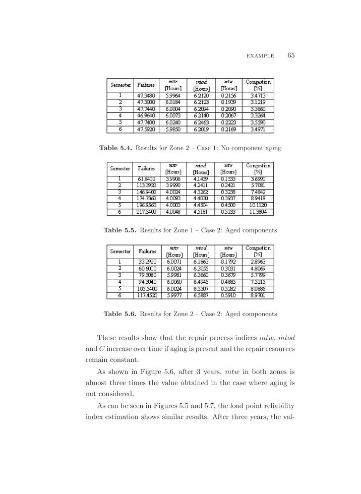
example 65
Table 5.4. Results for Zone 2 – Case 1: No component aging
Table 5.5. Results for Zone 1 – Case 2: Aged components
Table 5.6. Results for Zone 2 – Case 2: Aged components
These results show that the repair process indices mtw, mtod
and C increase over time if aging is present and the repair resources
remain constant.
As shown in Figure 5.6, after 3 years, mtw in both zones is
almost three times the value obtained in the case where aging is
not considered.
As can be seen in Figures 5.5 and 5.7, the load point reliability
index estimation shows similar results. After three years, the val-
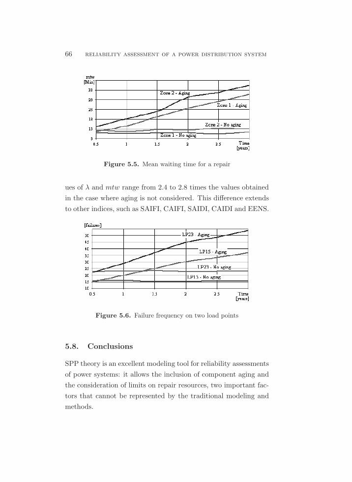
66 reliability assessment of a power distribution system
Figure 5.5. Mean waiting time for a repair
ues of λ and mtw range from 2.4 to 2.8 times the values obtained
in the case where aging is not considered. This difference extends
to other indices, such as SAIFI, CAIFI, SAIDI, CAIDI and EENS.
Figure 5.6. Failure frequency on two load points
5.8. Conclusions
SPP theory is an excellent modeling tool for reliability assessments
of power systems: it allows the inclusion of component aging and
the consideration of limits on repair resources, two important fac-
tors that cannot be represented by the traditional modeling and
methods.
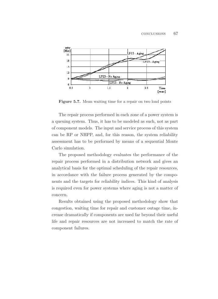
conclusions 67
Figure 5.7. Mean waiting time for a repair on two load points
The repair process performed in each zone of a power system is
a queuing system. Thus, it has to be modeled as such, not as part
of component models. The input and service process of this system
can be RP or NHPP, and, for this reason, the system reliability
assessment has to be performed by means of a sequential Monte
Carlo simulation.
The proposed methodology evaluates the performance of the
repair process performed in a distribution network and gives an
analytical basis for the optimal scheduling of the repair resources,
in accordance with the failure process generated by the compo-
nents and the targets for reliability indices. This kind of analysis
is required even for power systems where aging is not a matter of
concern.
Results obtained using the proposed methodology show that
congestion, waiting time for repair and customer outage time, in-
crease dramatically if components are used far beyond their useful
life and repair resources are not increased to match the rate of
component failures.


Chapter 6
Reliability Assessment of a
Protective Scheme
The aim of this chapter is to show the way protective systems are
incorporated into the proposed approach of modeling. Basically,
a method for the assessment of protective schemes is developed
here. It will be applied later in Chapter 8 to obtain a condensed
model of failures to operate of protective systems. The condensed
model will be used in the assessment of the power system.
The content of this chapter is taken from the paper “Reliabil-
ity Assessment of Protective Schemes Considering Time-Varying
Rates,” by Zapata, Kirschen, Torres and Rıos [28].
6.1. Introduction
The mission of a protective system (PS) is to detect abnormal
operating conditions in the protection zone (PZ) to which it is
assigned and to take actions that guarantee power system safety
and security and safeguard investment in power system assets.
Figure 6.1 shows the main types of protective system compo-
nents (PSC).
69
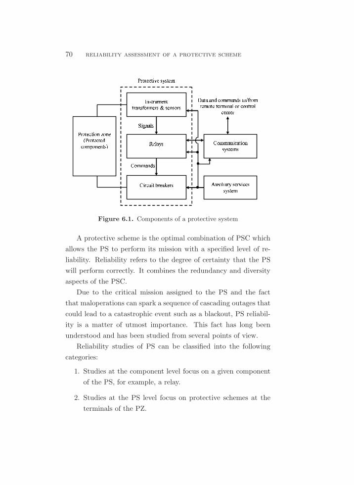
70 reliability assessment of a protective scheme
��������� ��������� �� ������������� ���������� ������������� ������� ��������� ����
���� ��� �� ���� ������ � �� �� ���� �� ������������������ ���� ������ ���������� �� � ������������������ ��� ��
Figure 6.1. Components of a protective system
A protective scheme is the optimal combination of PSC which
allows the PS to perform its mission with a specified level of re-
liability. Reliability refers to the degree of certainty that the PS
will perform correctly. It combines the redundancy and diversity
aspects of the PSC.
Due to the critical mission assigned to the PS and the fact
that maloperations can spark a sequence of cascading outages that
could lead to a catastrophic event such as a blackout, PS reliabil-
ity is a matter of utmost importance. This fact has long been
understood and has been studied from several points of view.
Reliability studies of PS can be classified into the following
categories:
1. Studies at the component level focus on a given component
of the PS, for example, a relay.
2. Studies at the PS level focus on protective schemes at the
terminals of the PZ.

problem statement 71
3. Studies at the power system level focus on the effects of PS
failures on power system reliability.
The study presented here focuses on studies of the second type.
They are helpful for:
• comparing design alternatives;
• assessing the effect of incorporating PSC with various levels
of reliability; and
• evaluating the impact of different preventive maintenance
strategies.
6.2. Problem Statement
Reliability assessments of protective schemes have been tradition-
ally performed under the assumption that PSC failure and repair
processes are stationary; this implies constant failure and repair
rates, constant probabilities of failure or constant availabilities.
Hence, the mathematical methods used for this task are those
that work under this assumption; for example, event trees, fail-
ure trees, reliability blocks and homogeneous exponential Markov
chains.
Although stationarity has long been a common assumption
in power system reliability, its relevance should be carefully re-
examined because of the growing importance of factors such as
aging, improvement/decrease in preventive maintenance and re-
pair resources, and the recognition that failure and repair rates
can be time-varying functions. If stationarity is no longer a valid
assumption, the application of the mathematical methods men-
tioned above is no longer valid. This chapter thus presents a
method on Stochastic Point Process (SPP) theory because this
approach can handle time-varying rates.

72 reliability assessment of a protective scheme
6.3. Failure Modes of a Protective System
A PS can take two kinds of actions: disconnection and connection
of the PZ. These actions can arise automatically, due to abnormal
operating conditions in the PZ, or manually, due to intentional or
unintentional orders given by an operator. These actions are ma-
terialized through the opening and closing of the circuit breakers
associated with the PZ. Requests to the PS to come into action
can thus be calls to open (CTO) or calls to close (CTC).
A PS operates correctly and appropriately if it does not fail
when it is called to operate and does not operate when this is
not required. The basic PS failure modes are failures to operate,
which include failures to open (FTO) and failure to close (FTC),
and false operations, which include false openings (FO) and false
closings (FC). Failures to operate include those situations where
the opening or closing takes more than the specified time.
Failures of PSC are classified here in accordance with their
potential effect on PS operation, viz., as FTO, FTC, FO and FC.
The term “potential” is used because the final effect of a PSC
failure on the PS operation depends on the configuration of the
protective scheme. Another type of PSC failure is the knocking
down (KND) which could lead to a situation where the PS does
not operate. All these failure modes do not necessarily apply to
every PSC.
6.4. Protective System Reliability Indices
6.4.1. Reliability
Reliability refers to the degree of certainty that the PS will per-
form correctly. It is measured as the ratio of wanted openings
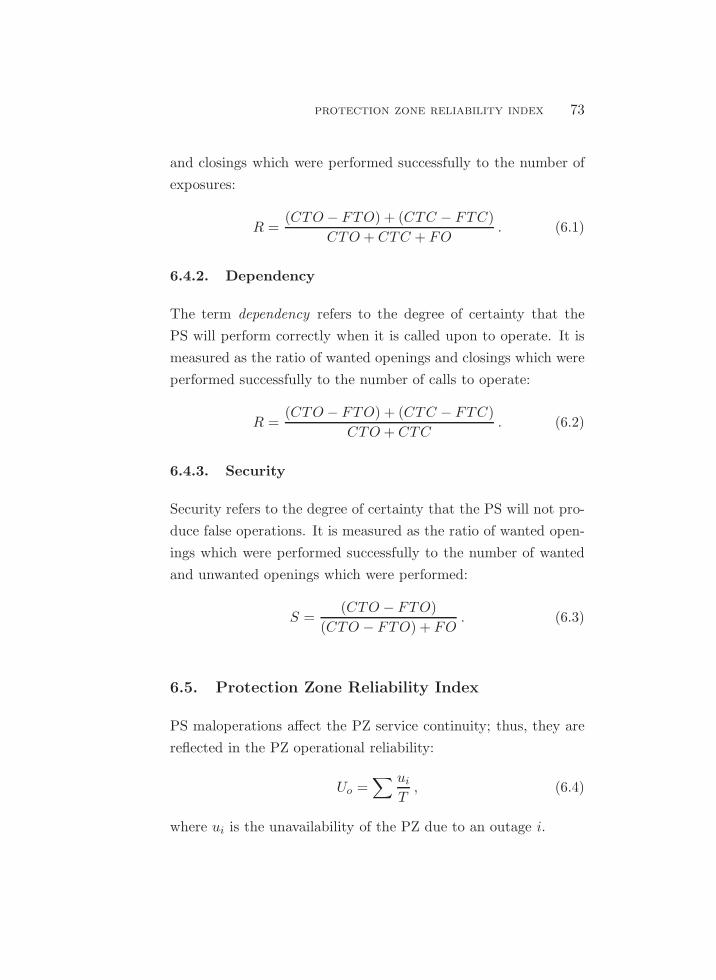
protection zone reliability index 73
and closings which were performed successfully to the number of
exposures:
R =(CTO − FTO) + (CTC − FTC)
CTO + CTC + FO. (6.1)
6.4.2. Dependency
The term dependency refers to the degree of certainty that the
PS will perform correctly when it is called upon to operate. It is
measured as the ratio of wanted openings and closings which were
performed successfully to the number of calls to operate:
R =(CTO − FTO) + (CTC − FTC)
CTO + CTC. (6.2)
6.4.3. Security
Security refers to the degree of certainty that the PS will not pro-
duce false operations. It is measured as the ratio of wanted open-
ings which were performed successfully to the number of wanted
and unwanted openings which were performed:
S =(CTO − FTO)
(CTO − FTO) + FO. (6.3)
6.5. Protection Zone Reliability Index
PS maloperations affect the PZ service continuity; thus, they are
reflected in the PZ operational reliability:
Uo =∑ ui
T, (6.4)
where ui is the unavailability of the PZ due to an outage i.

74 reliability assessment of a protective scheme
6.6. Proposed Method
6.6.1. Modeling
Each failure mode that applies to the PZ is represented by means
of an SPP model. These modes are: permanent faults, temporary
faults, and common mode faults between PZ and PS. Each failure
mode that applies to a given PSC is represented by means of an
SPP model. To obtain these models, failure data is divided based
on the failure mode, and the resulting sample data for each failure
mode is fitted to an SPP.
An SPP is fitted to the repair sample data corresponding to
each failure mode of the PSC and the PZ. It is assumed that repair
actions are perfect, i.e., that they effectively eliminate failures and
do not introduce new ones.
Preventive maintenance on the PZ and its PS include the ac-
tions performed by maintenance personnel and the auto-diagnostic
functions (self-check and monitoring) incorporated in some PSC,
such as relays. The time of occurrence of the events of these pro-
cesses is deterministic because they are programmed to occur at
fixed intervals; thus, they are generated using their yearly fre-
quency. Their duration is random and so it is modeled by means
of an SPP. Since these processes are not perfect in their function
of finding PSC failures, this feature is represented by means of E,
the probability of finding a PSC failure.
6.6.2. Reliability Assessment Procedure
The operation of the PS associated to a PZ is observed artificially
for a periodT of one or more years of interest by means of a pro-
cedure of a sequential Monte Carlo simulation (MCS).

proposed method 75
The application of MCS is justified by the fact that it is the
only method that can manage all probabilistic models of any type,
stationary and non-stationary, and also because it easily incorpo-
rates all actions which happen during the operating sequence of
a PZ and its PS, such as failures, repairs, maintenances, and self-
checks.
As depicted in Figure 6.2, a simulation consists of n artificial
observations of PS performance during T , under a scenario defined
by the protective scheme configuration, the failure and repair rates
and the strategy for preventive maintenance. The output of a
realization is the set of variables which allow computing the indices
of the PS model, viz., CTO, FTO, CTC, FTC and FO.
� � ����� � �� �� ��
� �� ���� ��� �� � �� ���� ��� ��
���� !�" #$Figure 6.2. General procedure of the reliability assessment algorithm

76 reliability assessment of a protective scheme
6.6.3. Procedure Inside a Realization
The procedure inside a realization is depicted in Figure 6.3. Each
downward arrow symbolizes the occurrence of a failure or main-
tenance in a PZ with a PS composed of PSC. The steps of this
procedure are:
1. Generate the failure process of PZ (f1 f2 . . . fn).
2. Generate the failure processes corresponding to each PSC.
3. Generate the process of preventive maintenance that requires
the disconnection of PZ (m1 m2 . . . mn).
4. Generate the processes of self-check, monitoring and preven-
tive maintenance on PSC that do not require the disconnec-
tion of PZ.
5. For each f − i or mi analyze if the PS operates correctly
for a CTO and a CTC, i.e., observe if PSC failures have
occurred before each call to operate and determine if they
lead to a PS failure to operate. Tie sets corresponding to the
request (CTO, CTC) and its origin (automatic, manual) are
used to determine PS success or failure. For FTO and FTC
it is assumed that PSC and PZ repairs can be performed
simultaneously; thus, PSC failures only add unavailability
to the PZ when they last more than PZ repairs.
6. For each PSC false opening generated whilst the PZ is in the
operating state, determine if the PS produces a trip. This
requires evaluating the tie sets which guarantee the trip can
be performed. Also analyze if the PS operates correctly when
CTC.
7. Repeat steps 1 to 6 n times.

proposed method 77
8. For each sub-period k (week, month, semester, year, etc.) of
T compute the indices of the PS failure model. When us-
ing time-varying rates, reliability indices should not be com-
puted for a single sub-period equal to T because variation is
lost.
������������������� ����� ��
� �
��� �����������
������� ������ �����⋮
Figure 6.3. General procedure inside a realization
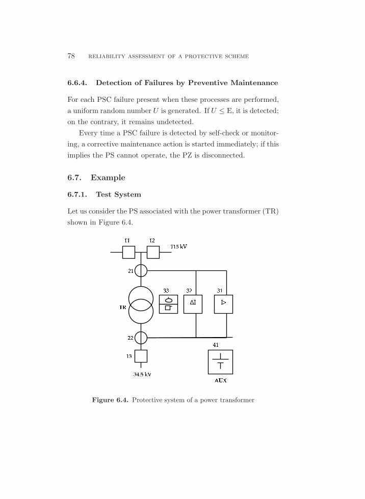
78 reliability assessment of a protective scheme
6.6.4. Detection of Failures by Preventive Maintenance
For each PSC failure present when these processes are performed,
a uniform random number U is generated. If U ≤ E, it is detected;
on the contrary, it remains undetected.
Every time a PSC failure is detected by self-check or monitor-
ing, a corrective maintenance action is started immediately; if this
implies the PS cannot operate, the PZ is disconnected.
6.7. Example
6.7.1. Test System
Let us consider the PS associated with the power transformer (TR)
shown in Figure 6.4.
∆���
����
������
���
���
���� ��
���� �� �
Figure 6.4. Protective system of a power transformer

example 79
This PS has three circuit breakers (11, 12 and 13), two current
transformers (21 and 22), an overcurrent relay (31), a differential
relay (32), a Buchholz relay (33) and auxiliary services (41).
The following PSC are not shown in Figure 6.4 but included in
the study: a 115 kV closing circuit (51), a 34.5 kV closing circuit
(52), a 115 kV opening circuit (61) and a 34.5 opening circuit (62).
Tables 6.1 and 6.2 show the reliability data for the PZ and the
PS, respectively. �λ ����� ����� ��� ��� ���� �������Table 6.1. Power transformer reliability data
Data for the opening/closing circuits were estimated from typ-
ical values; other data were estimated from indices obtained in
several reliability surveys performed in Colombia [19], [16].
6.7.2. Study Cases
1. Failure processes of PZ and PSC are modeled as HPP with
λ(t) = λF . Repair processes and preventive maintenance
durations are modeled as normal RP with λ(t) = 1/r. There
is only a preventive maintenance event per year with a mean
duration of 12 hours. E = 80% for FTO and FTC and
E = 10% for FO. This case reflects a situation where failure
and maintenance processes are stationary.
2. The failure processes of components 11, 12, 13, 31 and 32 are
modeled using a Power Law process with scale parameter λ
equal to the values for λF shown in Table 6.2 and shape pa-
rameter β = 1.2. The failure process of these components is
thus non-stationary with a positive tendency. Other models

80 reliability assessment of a protective scheme��� ��� ��� �� ���� ��λ =�����λ = �������λ = �������λ =���� !""# = !""# = $%&&' = ()**+ =����λ =�,-�λ = ���./��λ = ���01��λ =�2 3!""# =
3!""# =
3!""# =
3!""# =��,�λ = 4544667λ = 8 �����0�λ =�� 9:;;< =
9:;;< = 8 =>??@ =�,�λ =���λ = 8 ����0��λ =
�� 9:;;< =9:;;< = 8 =>??@ =����λ =����λ = 8 �������λ =
2� 9:;;< =9:;;< = 8 =>??@ =�A��λ = 4544B67λ = 8 ���1���λ =
2� 9:;;< =9:;;< = 8 =>??@ =����λ =�-���λ = 8 ���1C0�λ =
22 9:;;< =9:;;< = 8 =>??@ =�-���λ = D 8 DE� F!""# = D 8 DD D ����/G�λ = DH�H� D D F!""# = DI�I� D �-A�λ = D �����J�λ =D KLMMN = D KLMMN =
Table 6.2. Protective system reliability data
are the same as in case 1. This case reflects a situation of
aging and no strategy for improving preventive maintenance.
3. The same as in case 2, but now preventive maintenance fre-
quency is increased 100% each year. This case reflects a
situation of improving preventive maintenance to reduce the
effect of aging.
6.7.3. Results
Tables 6.3, 6.4 and 6.5 show the results for T = 3 years and
n = 10000 realizations. Figures 6.5 to 6.7 show R, D and S for
the cases studied. Simulations lasted 0.47 hours, 5.34 hours and
8.81 hours for cases 1, 2 and 3, respectively.

example 81���� � � � ���� � ������ � ���� �� �� ��� Table 6.3. Results for case 1 [%]���� � � � ����� !��"#$ %&�'� " $ �$� � ���& "'�� $#�#"" #�$ �' $��&"$! ���!��"�� $!�""! !�!%!$ #%���'' ���!''Table 6.4. Results for Case 2 [%]()*+ , - . /0123 4521674 89266:5 ;427488 32194:623 49256:1 832818: 4:2::5; 326446:23 8325196 892:773 83281;1 3257:6Table 6.5. Results for Case 3 [%]
Figure 6.5. Reliability of the protective system
6.7.4. Analysis of the Results
In the first case the PS reliability indices are constant because all
PSC failure and repair processes are stationary; thus, it is only
necessary to calculate them for one year.
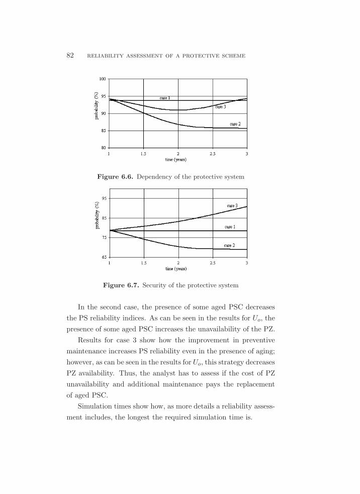
82 reliability assessment of a protective scheme
Figure 6.6. Dependency of the protective system
Figure 6.7. Security of the protective system
In the second case, the presence of some aged PSC decreases
the PS reliability indices. As can be seen in the results for Uo, the
presence of some aged PSC increases the unavailability of the PZ.
Results for case 3 show how the improvement in preventive
maintenance increases PS reliability even in the presence of aging;
however, as can be seen in the results for Uo, this strategy decreases
PZ availability. Thus, the analyst has to assess if the cost of PZ
unavailability and additional maintenance pays the replacement
of aged PSC.
Simulation times show how, as more details a reliability assess-
ment includes, the longest the required simulation time is.

Conclusions 83
6.8. Conclusions
A new method for reliability assessment of protective schemes is
presented in this work. Unlike traditional methods, it supports
the consideration of time-varying failure and repair rates, and di-
verse maintenance strategies. However, the great improvement in
modeling detail offered by this method has a price—the long com-
putational time required by the simulation. Thus, its application
is only recommended for those situations involving time-varying
rates, for otherwise it is simpler and faster to apply the traditional
methods.
This method can also be easily extended to reliability assess-
ment of small portions of a power system such as substations.


Chapter 7
Reliability Assessment of a
Substation
The aim of this chapter is to apply the method of stochastic point
process modeling and a sequential Monte Carlo simulation to the
assessment of a small portion of a power system. This assessment
includes the protective system associated to each main power sys-
tem component.
The content of this chapter is taken from the paper “ Relia-
bility Assessment of Substations Using Stochastic Point Processes
and Monte Carlo Simulation,” by Zapata, Alzate and Rıos [18].
7.1. Introduction
Electrical power substations are the most critical parts of a power
system, for it is there where the main power system components
interconnect. A substation failure can produce the outage of many
power system components, which can be disastrous for the system.
For this reason, substation reliability is a matter of outmost im-
portance.
Reliability of a substation depends on:
• The substation configuration, i.e., the arrangement of circuit
85

86 reliability assessment of a substation
breakers or busbars.
• The reliability of substation components.
• The reliability of protective systems.
A substation reliability assessment evaluates the effect of these
aspects on the service continuity of the main power system com-
ponents connected to the substation.
7.2. Motivation
The following aspects motivated the development of the proposed
method:
7.2.1. The Necessity of Considering Time Varying Rates
Reliability assessments of substations has been traditionally per-
formed under the assumption that the failure and repair processes
of substation components are stationary; it is expressed by means
of constant event rates, constant probabilities of failure or constant
availabilities.
This practice is also reflected in the mathematical methods
that have been applied for this task: cut sets, reliability blocks,
homogeneous Markov chains, fault trees, etc. However, nowadays
the application of this assumption ought to be carefully examined
because, due to factors such as aging, improvement/decrease on
preventive maintenance and repair resources, the failure and repair
rates of substation components can be time-varying functions.
In order to manage time-varying rates with the traditional
methods, the analyst has the following options:
1. To manually change the input parameters (event rates, fail-
ure probabilities, availabilities) to the expected values for the
motivation 87
future years under several scenarios of improvement/deterioration
of component reliability, preventive maintenance and repair
process performance. However, this approach is not very ac-
curate because event rates do not change in discrete steps
but continuously.
2. To incorporate the functions which represent the time-varying
rates into a non-homogeneous Markov process. However,
this method has problems for adjusting the operating times
and of tractability for some types of time-varying rates.
Thus, the proposal here is to model the failure and repair pro-
cesses of substation components by means of SPP. It allows the
utilization of time-varying rates in an easier way than in the non-
homogeneous Markov chain method.
7.2.2. The Necessity of Including the Effect
of Protective Systems
It has been a common practice for reliability assessments of sub-
stations to only consider the primary plant components, i.e., the
high-voltage ones, and assume the effect of items of secondary
plant such as protective components, auxiliary services, communi-
cation systems, cablings, etc. are included in the reliability models
of the high-voltage ones.
Regarding this practice, Dortolina et al. [5] pointed out that:
“There are practical situations where it would be
important to explicitly evaluate the influence of the pro-
tective relaying equipment on the overall substation re-
liability. These include: (i) Evaluating the effect of a
given protective scheme on the reliability of different
substation arrangements, and (ii) evaluating the effect

88 reliability assessment of a substation
of the redundancy of the protective relaying equipment
on the reliability of a given (and perhaps existing) sub-
station.”
This practice is in part justified by the fact that all analytic
methods for reliability assessment that allow a detailed system
representation require an exhaustive list of operating states; thus,
if many components are considered, the amount of system operat-
ing states becomes huge. On the other hand, the proposal here is
to perform the reliability assessment by means of a procedure of
sequential MCS. This allows including as many components and
operating conditions as the analyst wants and does not require an
exhaustive list of system operating states.
7.3. Concept of Protection Zones
Each main power system component (transmission line, power
transformer, reactive compensation, busbar) connected to a sub-
station defines a protection zone (PZ); this concept is illustrated
in Figure 7.1.
Each PZ has a protective system (PS) composed of several pro-
tective system components (PSC); PSC include circuit breakers,
disconnectors, instrument transformers, relays, trip circuits, etc.
Communication and auxiliary service systems can be part of each
PS or shared by several of them.
7.4. Failure Modes of Protected Zones
Failures of PZ can be:
(i ) Permanent: Those failures that have to be repaired by
maintenance personnel.

common mode failures 89
��������������
�������������� �������������� ��������������� �
Figure 7.1. Protection zones associated to a single busbar substation
(ii ) Temporary: Those failures that disappear without tak-
ing any repair action; thus, the PZ is reconnected by
means of an automatic reclosing action.
7.5. Common Mode Failures
Common mode failures are those that simultaneously affect PZ
and PSC. Most of these kinds of failures are permanent.
7.6. Tie Sets
In the proposed method, every time a PS is called to operate, or
a PSC produces a false opening, the PS outcome is determined
using tie sets.
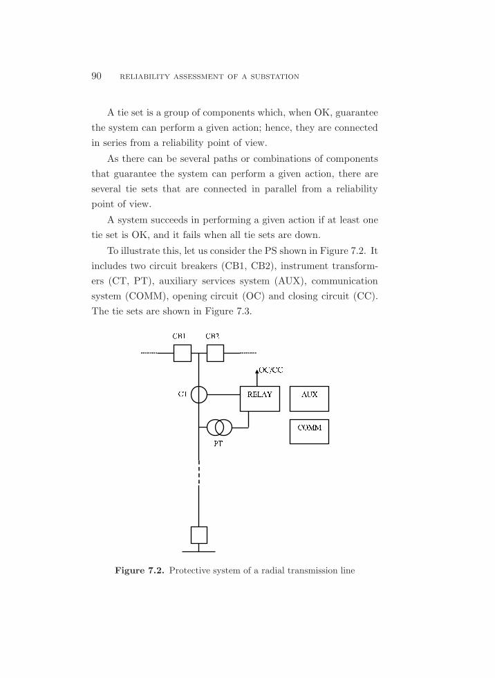
90 reliability assessment of a substation
A tie set is a group of components which, when OK, guarantee
the system can perform a given action; hence, they are connected
in series from a reliability point of view.
As there can be several paths or combinations of components
that guarantee the system can perform a given action, there are
several tie sets that are connected in parallel from a reliability
point of view.
A system succeeds in performing a given action if at least one
tie set is OK, and it fails when all tie sets are down.
To illustrate this, let us consider the PS shown in Figure 7.2. It
includes two circuit breakers (CB1, CB2), instrument transform-
ers (CT, PT), auxiliary services system (AUX), communication
system (COMM), opening circuit (OC) and closing circuit (CC).
The tie sets are shown in Figure 7.3.
�������� ���� ����� ������
Figure 7.2. Protective system of a radial transmission line
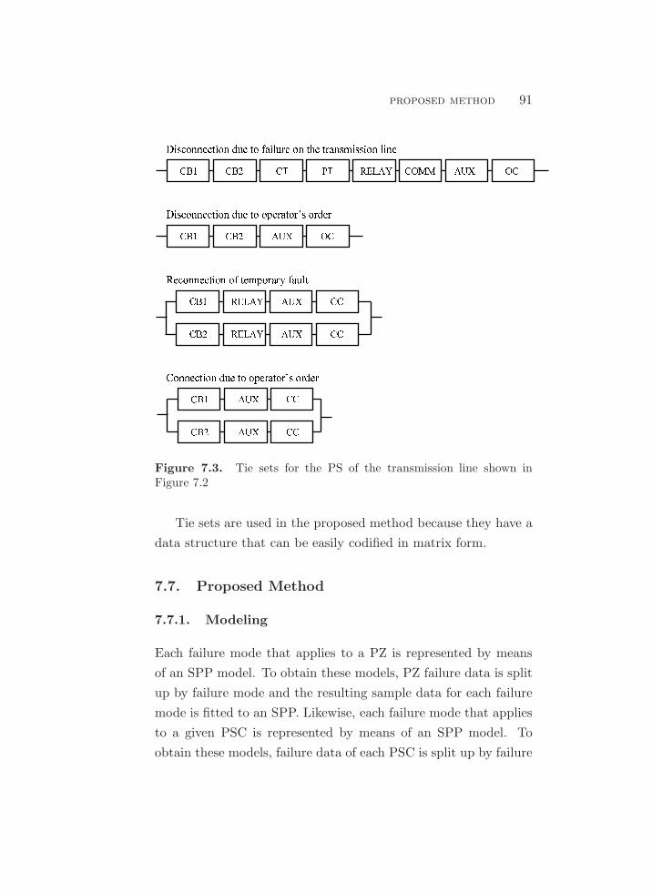
proposed method 91
���������� ��� �� ������ ���
�� ���������� ��� �� ������ �� ��� ��� �� ��� ������ ���������� ��� �� ������ ������ ��� ��� �������������� �� ������ �������� ���� ��� ����� ���� ��� ����� ��� ����� ��� ��
��� ��� �! "! ���� ��## �����
Figure 7.3. Tie sets for the PS of the transmission line shown inFigure 7.2
Tie sets are used in the proposed method because they have a
data structure that can be easily codified in matrix form.
7.7. Proposed Method
7.7.1. Modeling
Each failure mode that applies to a PZ is represented by means
of an SPP model. To obtain these models, PZ failure data is split
up by failure mode and the resulting sample data for each failure
mode is fitted to an SPP. Likewise, each failure mode that applies
to a given PSC is represented by means of an SPP model. To
obtain these models, failure data of each PSC is split up by failure

92 reliability assessment of a substation
mode and the resulting sample for each failure mode is fitted to
an SPP.
Each common mode failure is represented by means of an SPP
model. Data samples to obtain these models are taken from PZ
and PS failure data.
An SPP is fitted to the repair sample data corresponding to
each failure mode. It is assumed that repair actions are perfect,
i.e., they effectively eliminate failures and do not introduce new
ones.
For FTO and FTC it is assumed that PSC and PZ repairs can
be performed simultaneously; thus, PSC failures only add unavail-
ability to the PZ when they last more than PZ repairs.
Preventive maintenance on PZ and PS include the actions per-
formed by maintenance personnel and the auto-diagnostic func-
tions (self-check and monitoring) incorporated in some PSC, such
as relays. The time of occurrence of the events of these processes
is deterministic because they are programmed in the form of fixed
intervals; thus, they are generated using their yearly frequency.
Their duration is random and so they are modeled by means of
an SPP. These processes are not perfect in their function of find-
ing PSC failures; this feature is represented by means of E, the
probability of finding a PSC failure.
7.7.2. Reliability Assessment Procedure
The operation of each PZ and its associated PS is observed artifi-
cially for a period T of one or more years of interest by means of
a procedure of sequential MCS.
A simulation consists of n artificial observations of the operat-
ing sequence of PZ and PS under a scenario defined by substation
configuration, protective scheme configuration, failure and repair

proposed method 93
rates, and strategy for preventive maintenance. FC are not con-
sidered because they do not affect PS operation.
7.7.3. Procedure Inside a Realization
The procedure inside a realization is depicted in Figure 7.4. Each
downward arrow symbolizes the occurrence of an event of failure
or maintenance in a PZ with a PS composed of X PSC.
����������� ���� ���� ��
� �
���������� ����
� ������������� ����⋮
������
Figure 7.4. General procedure inside a realization

94 reliability assessment of a substation
Steps are:
1. Generate the PZ failure process (f1 f2 . . . fn).
2. Generate the failure processes corresponding to each PSC.
3. Generate the process of preventive maintenance that requires
the PZ disconnection (m1m2 . . . mn).
4. Generate the processes of self-check, monitoring and pre-
ventive maintenance on PSC which does not require the PZ
disconnection.
5. For each fi or mi analyze if the PS operates correctly when
CTO and CTC; i.e., observe if PSC failures have occurred
before each call to operate and determine if they lead to a
PS failure to operate.
6. If the PS fails to operate, determine if the PS that give
local back up operate correctly and the additional PZ that
were disconnected. Determine the effect of PS failure in PZ
availability.
7. For each PSC false opening that has been generated while
PZ is in the operative state, determine if the PS produces a
trip. This is performed evaluating the tie sets which guar-
antee that the trip can be performed. Also analyze if the PS
operates correctly when CTC. Determine the effect of false
opening in PZ availability.
8. Repeat steps 1 to 7 n times or after reaching other stopping
rule.
9. For each sub-period k (week, month, semester, year, etc.) of
T compute the indices of the PZ. When using time-varying

proposed method 95
rates, reliability indices should not be computed for a single
sub-period equal to T because variation is lost.
7.7.4. Detection of Failures by Preventive Maintenance
For each PSC failure that is present when these processes are per-
formed, a uniform distributed random number U is generated. If
U ≤ E, it is detected; on the contrary, it remains undetected.
7.7.5. Reliability Indices
Substation reliability is measured by means of indices related to
the service continuity of each PZ. These are expected event rates,
expected availability and expected unavailabilities.
Definitions:
o : An outage event, i.e., a PZ disconnection.
u : Down time due to an outage.
f : A PZ outage due to a failure in this zone or in an
upper hierarchical PZ.
m : A PZ outage due to a preventive maintenance action
in this zone or in an upper hierarchical PZ.
fo : A PZ outage caused by a false opening originated in
its own PS or in a one of an upper hierarchical PZ.
bu : A PZ outage caused by a backup action taken by its
own PS or by a one of an upper hierarchical PZ.
• Expected operational outage rate:
λo =
∑
(f +m+ fo+ bu)
T −∑
u. (7.1)
• Expected operational unavailability:
Uo =∑ u
T. (7.2)
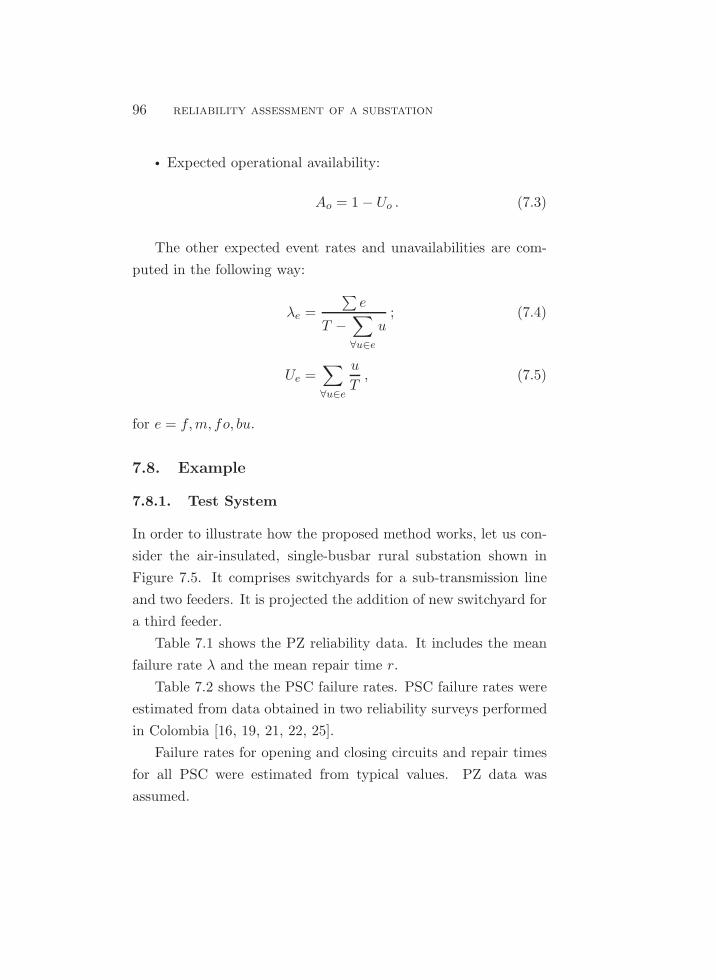
96 reliability assessment of a substation
• Expected operational availability:
Ao = 1− Uo . (7.3)
The other expected event rates and unavailabilities are com-
puted in the following way:
λe =
∑
e
T −∑
∀u∈e
u; (7.4)
Ue =∑
∀u∈e
u
T, (7.5)
for e = f,m, fo, bu.
7.8. Example
7.8.1. Test System
In order to illustrate how the proposed method works, let us con-
sider the air-insulated, single-busbar rural substation shown in
Figure 7.5. It comprises switchyards for a sub-transmission line
and two feeders. It is projected the addition of new switchyard for
a third feeder.
Table 7.1 shows the PZ reliability data. It includes the mean
failure rate λ and the mean repair time r.
Table 7.2 shows the PSC failure rates. PSC failure rates were
estimated from data obtained in two reliability surveys performed
in Colombia [16, 19, 21, 22, 25].
Failure rates for opening and closing circuits and repair times
for all PSC were estimated from typical values. PZ data was
assumed.

example 97
��� � ���� �� ������ ����� �
����� �
������ �
����� � ����� �
����� � ��� ��������� � ������ � ������ �
� �� ������������ �� !� " �����
∆#�
Figure 7.5. Test system
Table 7.1. Reliability data of protection zones
Table 7.2. Failure rates of protective system components [failures/year]

98 reliability assessment of a substation
Preventive maintenance frequency is one event per year in each
zone. E = 80% for FTO and FTC, and E = 20% for FO. Existent
relays do not incorporate auto-diagnostic functions.
The mean duration of preventive maintenance events is r = 12
hours.
It is assumed the PZ failure processes are stationary and that
existent circuit breakers and relays are aged. All stationary failure
processes are modeled by means of HPP with λ(t) = λ. The failure
processes of aged components are modeled by means of a Power
Law process with scale parameter equal to λ and shape parameter
β = 1.2.
Repair processes and preventive maintenance durations are
modeled as normal RP with λ(t) = 1/r and variance of 50%,
r = 8 hours for high-voltage switchgear, opening/closing circuits
and auxiliary services and r = 4 hours for protective relays.
7.8.2. Study Cases
1. A reliability assessment considering the real reliability con-
dition of the components.
2. A reliability assessment considering that all PSC failure pro-
cesses are stationary.
The study focuses on the substation reliability indices seen at
the connection point of the new feeder.
7.8.3. Results
Tables 7.3 to 7.6 show the reliability indices for the new bay
with years and simulations of n = 10000 realizations. Figures 7.6
and 7.7 show and for the study cases.

example 99
Required time for simulating these cases was in average 24 hours
using common desktop computers (Intel Core 2 processor, 2.4 and
2.66 GHz, 2 to 3 GB of RAM).
Table 7.3. Expected event rates in [events/year] for PZ5 – Case 1
Table 7.4. Expected unavailabilities in [%] for PZ5 – Case 1
Table 7.5. Expected event rates in [events/year] for PZ5 – Case 2
Table 7.6. Expected unavailabilities in [%] for PZ5 – Case 2
7.8.4. Analysis of the Results
Results of case 1 show that although PZ5 has new substation
equipment, its reliability indices increase over time due to the
presence of aged substation equipment in the other bays.
On the other hand, for most term of the study, the reliability
indices obtained in case 2 are lower than those obtained in case 1.
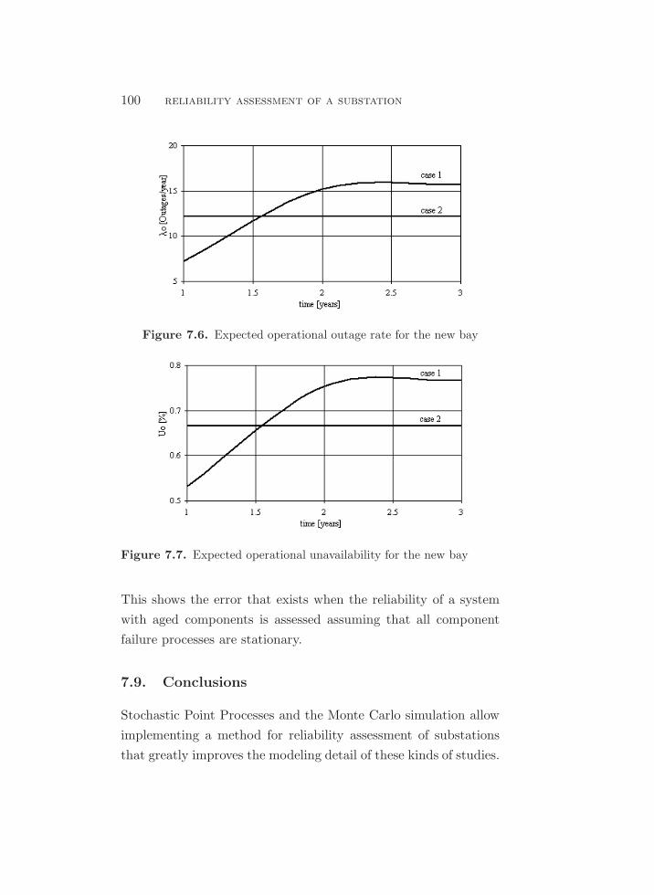
100 reliability assessment of a substation
Figure 7.6. Expected operational outage rate for the new bay
Figure 7.7. Expected operational unavailability for the new bay
This shows the error that exists when the reliability of a system
with aged components is assessed assuming that all component
failure processes are stationary.
7.9. Conclusions
Stochastic Point Processes and the Monte Carlo simulation allow
implementing a method for reliability assessment of substations
that greatly improves the modeling detail of these kinds of studies.

conclusions 101
It can manage time-varying rates and allows a detailed representa-
tion of the protective systems operating sequence and the effect of
their failures. Additionally, it does not require an exhaustive list
of operating states as other methods do. However, this improve-
ment in modeling detail has a price—the long computational time
required by the simulation.


Chapter 8
Modeling of Failures to
Operate of Protective
Systems for Reliability
Studies at the Power System
Level
The aim of this chapter is to present the method for obtaining a
condensed model of protective system failures to operate that will
be incorporated in the assessment of the power system. The facts
that justify this kind of representation are also discussed.
The content of this chapter is taken from the paper “Modeling
of Protective System Failures to Operate for Reliability Studies
at the Power System Level Using Stochastic Point Processes,” by
Zapata, Kirschen, Torres and Rıos [30].
8.1. Power System Reliability Assessments
Considering PS Failures to Operate
To illustrate how a power system reliability study that considers
PS failures to operate works, let us consider the PS at each trans-
103

104 reliability studies at the power system level
mission line terminal in the power system shown in Figure 8.1,
which has the scheme shown in Figure 8.2.
����� ��� ���
������ �� �
���
�� �� �
��������� ������� ���������� �� � �� ���������! "
Figure 8.1. Analysis on the effect of protective system failures to open
#$%&%' (' )*+#,%-..
Figure 8.2. Protective system at a terminal of a transmission line

assessments considering ps failures to operate 105
For a fault on line L1, it is necessary to analyze if the PS at
terminals 1 and 3 operate correctly, i.e., if they open. If the PS
at terminal 3 FTO, it is then necessary to analyze if the PS at
terminals 2, 4 and 6 of transmission lines L3, L5 and L7, respec-
tively, operate correctly, and so on. Thus, for this kind of study,
it is necessary to represent the PS associated to each PZ. There
are two main approaches for this task:
1. To incorporate the reliability models of the PSC associated
to each PS.
2. To condense the effect of all PSC associated to a given PS
into the reliability models of the circuit breakers associated
to the PZ. This can be done because all PS failures are re-
flected on the PZ circuit breakers, no matter the PSC that
caused them.
The first approach is the less popular one because it demands
more computer processing capacity (RAM) and computing time,
due to the huge number of reliability models that have to be eval-
uated. To illustrate this, let us consider a reliability study of the
power system shown in Figure 8.1. If it only considers failures
on the transmission lines, it will require 16 failure models (8 for
permanent failures + 8 for temporary failures). If it also considers
FTO, it is necessary to incorporate 224 additional failure mod-
els in the first approach, but only 16 in the second one. These
numbers are obtained in the following way:
• 224 = (8 transmission lines) ∗ (2 terminals per transmission
line) ∗ (7 PSC per PS) ∗ (2 failure modes per PSC (FTO +
KND));
• 16 = (8 transmission lines) ∗ (2 terminals per transmission
line) ∗ (1 circuit breaker per terminal).

106 reliability studies at the power system level
A common practice in the first approach is to restrict the analy-
sis to the PSC considered “most important,” viz., circuit breakers,
current transformers and relays; however, this also decreases the
level of detail of the reliability study.
Regarding the second approach, the condensed model at each
circuit breaker is expressed in the form of a probability for each
type of PS failure to operate. These probabilities are computed
before and out of the power system reliability study, using operat-
ing data or by means of a reliability assessment of the protective
scheme.
The second method of obtaining the probabilities of the con-
densed model is applied in those situations where the aim is to
evaluate the impact of incorporating PSC with different levels of
reliability and of considering diverse protective schemes.
8.2. Problem Statement
Several modeling tools have been applied to obtain a condensed
model of PS failures to operate: homogeneous Markov chains,
event trees, fault trees, cut sets and reliability blocks. All of them
work under the assumption that PSC failure and repair processes
are stationary; this is expressed by means of constant failure and
repair rates, constant probabilities of failure or constant availabil-
ities.
Although stationarity has long been a common assumption
in power system reliability, its relevance should be carefully re-
examined, due to the growing importance of factors such as aging
and improvement/decrease in maintenance resources. If station-
arity is no longer a valid assumption, the application of the math-
ematical methods mentioned above is no longer valid. For this
reason, this author has proposed a method based on SPP model-

proposed method 107
ing that can manage constant or time-varying rates. It is applied
here for obtaining the condensed model of a PS.
8.3. Proposed Method
Using the assessment procedure described in Chapter 6, the prob-
abilities of the condensed model are computed in the following
way:
P [FTO]lk =FTOk
CTOk; (8.1)
P [FTC]lk =FTCk
CTCk. (8.2)
8.4. Example
Consider the test system presented in Chapter 6 and the same
study cases. Tables 8.1 to 8.3 show the results for T = 3 years
and n = 10000 realizations. Figure 8.3 shows the probability of
FTO at circuit breaker 13 for the three study cases.
Simulations lasted 0.47 hours, 5.34 hours and 8.81 hours for
cases 1, 2 and 3, respectively. The post-processing of the simula-
tion outputs to compute the probabilities of the condensed model
lasted less than fifteen minutes in all study cases.��������� ��� � ��� ��� � ��� ��� � ��� �� ��� �� ���− �� ��� � !"#
− $% $&' () *+,− -- -. -/0 12 345
− −678 9 :78 878;<; 878;=> 878:>< 878888 878888 878888 8788<8
Table 8.1. FTO probability of the protective system – Case 1

108 reliability studies at the power system level��������� ��� � ��� ��� � ��� ��� � ��� �� ��� �� ���− �� ��� � !"#
− $% $&' () *+,− -- -. -/0 12 345
− −678 8789:8 878969 878:;< 878888 878888 878888 8788=6:78 8768=6 878>?= 878@:< 878888 878888 878888 8786>6?78 8766>> 8768=8 878@?= 878888 878888 878888 8786;:
Table 8.2. FTO probability of the protective system – Case 2ABCDEFGHIJK LLM NO PQR LSM NO PQR LTM NO PQR UU UVW XY Z[\− ]] ]_ `a bcd
− ef egh ij klm− nn no npq rs tuv
− −wxy yxyzw{ yxyzw| yxy}~z yxyyyy yxyyyy yxyyyy yxyy�w}xy yxy�{~ yxy�}y yxyz|w yxyyyy yxyyyy yxyyyy yxywwy|xy yxyzwy yxyzy} yxy}�| yxyyyy yxyyyy yxyyyy yxyy�y
Table 8.3. FTO probability of the protective system – Case 3
Figure 8.3. FTO probability at circuit breaker 13
8.5. How to Use this Model
To illustrate how the PS condensed model is applied, let us con-
sider the sketch shown in Figure 8.4.
For a given PS failure mode, for example FTO, the probabili-
ties of occurrence of a FTO at each circuit breaker at a given time
are a part of the total probability of the sample space. The sample
space also includes the event of not occurrence of FTO.
To sample this model in the reliability assessment at the power
system level, a U is generated each time a failure affects the PZ; the
value of U defines the event that occurs. For example, using data
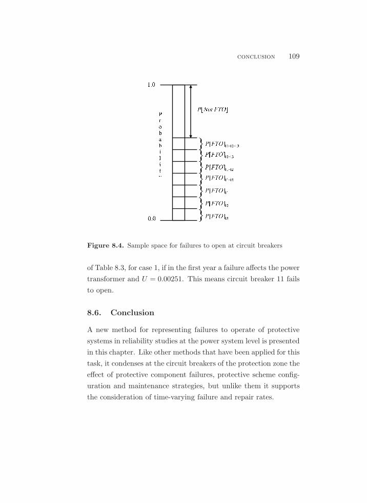
conclusion 109
�����������
��
��� �� ��� ��� �� ��� ��� �� ��� �� �� !" #$%−�� �& !" #$%−
'( ')* +, -./−
0 12 345 678
} } } } } } } 99 9: 9;< => ?@A− −
Figure 8.4. Sample space for failures to open at circuit breakers
of Table 8.3, for case 1, if in the first year a failure affects the power
transformer and U = 0.00251. This means circuit breaker 11 fails
to open.
8.6. Conclusion
A new method for representing failures to operate of protective
systems in reliability studies at the power system level is presented
in this chapter. Like other methods that have been applied for this
task, it condenses at the circuit breakers of the protection zone the
effect of protective component failures, protective scheme config-
uration and maintenance strategies, but unlike them it supports
the consideration of time-varying failure and repair rates.


Chapter 9
The Loss of Component
Scenario Method to Analyze
the Vulnerability of a
Composite Power System
This chapter presents the method for assessing the vulnerability
of a composite power system. It gathers all the concepts and
methods presented in previous chapters.
Most of the content of this chapter is taken from the paper “A
Method for Studying Loss of Component Scenarios in a Power
System Using Stochastic Point Processes,” by Zapata, Torres,
Kirschen and Rıos [27].
9.1. Definition of Loss of Component Scenario
A loss of component scenario (LCS) is the situation where a power
system with n components has x components out of service due
to planned or unplanned events. It is denoted as a n−x LCS and
it is called an LCS of order x.
A high-order LCS is defined here as the situation where x > 2.
111

112 vulnerability of a composite power system
Only failures that force components to the unavailable state
or derate their capacity are considered here as unplanned events.
Planned events are not considered, because they can be programmed
for a time when system reliability is not affected.
As an example, consider the small system shown in Figure 9.1.
It has 7 components, 128 operating states, 7 n− 1 LCS, 22 n− 2
LCS, etc.
�
���
⋮
⋮
⋮
�� −
�� −
�� −
�� −
Figure 9.1. Operating states of a small power system
A component is defined as an item of primary plant of the
power system (e.g., transmission lines, transformers and generat-
ing units) or an item of secondary plant (e.g., auxiliary services
objective of an lcs study 113
systems and protective relays). Thus, component failure models
include failures of both types If each component has two states,
“available” and “unavailable;” the state space of operating states
of a system with n components has a dimension of 2.
The term operating state refers here to an LCS and does not
qualify the system operating condition in terms such as “Normal,”
“Alert,” or “Emergency,” as used in the context of power system
security.
Because every power system has many components, the dimen-
sion of the space of operating states is huge; hence, every study
on the occurrence of LCS is a cumbersome task, no matter the
assessment method applied.
9.2. Objective of an LCS Study
The aim of this study is to measure the occurrence of LCS by
means of the following indices:
• the probability of occurrence Pn−x;
• the expected frequency Fn−x; and
• the mean duration Dn−x.
Although this objective may appear similar to the one of the
reliability assessment technique called “state enumeration,” the
difference is that in the present study the indices are determined
globally for the set of operating states that belong to a given LCS
order and not for each of them separately.
For example, considering the system shown in Figure 9.1. LCS
indices are calculated for the n−2 LCS order and not for each one
of the 22 operating states that belong to this order.

114 vulnerability of a composite power system
9.3. Traditional Modeling for Reliability Studies
For simplicity, in the following discussion, only the basic compo-
nent reliability model of two operating states shown in Figure 9.2
is considered. However, the proposed method extends to models
with any number of states.
�����
������
λ
µ
Figure 9.2. Two-state component reliability model
This model is defined by means of a failure rate λ and a repair
rate µ, which can be estimated from operating records that cover
a period T in the following way:
λ =1
ttf=
nf
T −∑nr
j=1 ttri, (9.1)
µ =1
ttr=
nr
T −∑nf
j=1 ttfi, (9.2)
where ttf , nf , ttr and nr denote respectively the time to failure, the
number of failures, the time to repair and the number of repairs.
Over-lined symbols such as x denote the statistical mean of the
variable.
Two important component reliability indices are the availabil-
ity (A) and the unavailability (U = A), which can be estimated

traditional modeling for reliability studies 115
from operating records in the following way:
A = P1(∞) =µ
λ+ µ=
1
T
nf∑
j=1
ttfj , (9.3)
U = P2(∞) =λ
λ+ µ=
1
T
nr∑
j=1
ttrj , (9.4)
where Pi(∞) denotes the probability of finding state i in the long
run. Constant failure and repair rates imply that the failure and
repair processes are stationary and hence, in the long run, A and
U tend towards the estimates (9.3) and (9.4) independently of the
probability distribution of ttf and ttr.
If the distributions of ttf and ttr of all components are expo-
nential, the LCS study can be solved using the continuous Markov
chain method. Figure 9.3 shows a Markov chain representation for
a system with n components.
The mathematical formulation of this method for a system of
n components is the set of ordinary differential equations:
[P ]t = [M ]t[P ]t , (9.5)
where [P ] is a vector with the probabilities of the n∗n states, and
is the matrix of transition rates between states.
If k operating states are LCS of order x the probability of
occurrence of LCS of this order is:
Pn−x =k
∑
j=1
Pj(∞) . (9.6)
The expected frequency and the mean duration of LCS of order

116 vulnerability of a composite power system
�� −
…
…
⋮
�
��
�� − �� −
−
…
Figure 9.3. Markov chain diagram for the state space of system oper-ating states
x are computed as:
Fn−x = Pn−x ∗∑
h , (9.7)
Dn−x =1
∑
h, (9.8)
where∑
h is the sum of the rates of all the transitions leaving
states belonging to an LCS of a particular order, i.e., the transi-
tions that cross one of the dashed lines in Figure 9.3.
If the failure and repair processes of all components are in-
dependent, it is not necessary to solve (9.5) first to apply (9.6).
Each term of (9.6) can be obtained by applying the formula of

what do the assumptions of traditional modeling
imply? 117
simultaneous occurrence of independent events (Ei):
P [E1 E2 . . . EN ] =N∏
j=1
P [Ej ] . (9.9)
where Ei denotes the operating state (Ai or Ai) of component i.
If all component failure and repair processes are stationary and
independent, (9.9) is valid no matter the probability distributions
used to represent these processes.
It is important to observe that (9.9) does not apply for the
case where common failure modes exist and its extension to include
them is very complicated. In this case, common failure modes have
to be included in M , which can then be solved by applying (9.5).
It is also important to point out that before the application of (9.5)
or (9.9), a list of all possible operating states has to be elaborated
and this is not an easy task.
9.4. What Do the Assumptions of Traditional
Modeling Imply?
9.4.1. Stationary Failure and Repair Processes
Stationarity of failure and repair processes has been a common
assumption in the field of power system reliability. However, the
validity of this assumption must be examined carefully, especially
for the failures. Because of component aging and lack of preven-
tive maintenance—two conditions currently present in many power
systems all over the world—component failure rates may not be
constant but rather increasing functions of time.
On the other hand, a constant repair rate means that the per-
formance of repair teams is not affected by internal or external
factors. However, in real life, crew performance is affected by ex-

118 vulnerability of a composite power system
ternal factors such as weather and traffic, as well as by internal
factors such as available tools and personnel skills.
Non-constant failure and repair rates also mean that the study
of LCS cannot be done by applying (9.3) to (9.9). One way of
overcoming this problem is to introduce time-varying rates into M
to solve (9.5), i.e., by making it into a non-homogeneous Markov
chain process. However, this kind of process has problems with the
adjustment of the operating times and with tractability for some
types of time-varying rates. Even if the limitations of the non-
homogeneous Markov chain process were considered unimportant,
this kind of modeling has another drawback that is discussed next.
9.4.2. Independent Component Repair Processes
It has also been a common practice in the field of power system
reliability to include repairs as part of component models; this
approach means that:
1. The repair process of each component is independent of the
repair processes of other components.
2. Repair resources are unlimited because every time a compo-
nent fails it is immediately repaired. This is equivalent to
assuming that each component has a dedicated repair team.
Obviously, these assumptions are unrealistic. For maintenance
purposes, a power system is typically split into maintenance zones
which are assigned to repair teams. Repair resources are limited
because crews have to fix all failed components located in their
zone. Hence, some failures have to wait until the ones that oc-
curred first are repaired. Thus, repairs of component located in a
given maintenance zone are not independent.
proposed method 119
9.4.3. Proposal
To improve the modeling flexibility of the LCS study, it is proposed
to represent the component failure processes using an SPP and the
repair process of each maintenance zone of the power system using
concepts from queuing theory.
9.5. Proposed Method
9.5.1. Failure Process Modeling
9.5.1.1. Components with Two Operating States
The failure process of a two-state component is represented by
means of an SPP model.
9.5.1.2. Components with More than Two Operating States
Some people believe components with more than two operating
states cannot be represented by SPP. This is not true. In this
case, the component is represented by one SPP model for each
operating state (rated, derated and failed states).
For example, consider the Markov chain model for a power
transformer with a forced cooling system shown to the left in Fig-
ure 9.4. λ1(t) is the forced failure rate and λ2(t) the failure rate
of the forced cooling system. In this case, the failure process of
the power transformer is represented by two independent SPP as
shown to the right in Figure 9.4.
9.5.1.3. Common Mode Failures
Each common failure mode is represented by means of an SPP
model. This means that common mode failures have to be dis-
tinguished from other types of component failures. Because the

120 vulnerability of a composite power system
��� �������� λ ��
��� �������
� ��������� �������� �� ��λ
� ! "#λ
λ$% &' µ$% &'
µ �� ������ ���()*��+���, -�)(����
Figure 9.4. SPP modeling for a component with three operating states
definition of SPP imposes that only one event can occur at any
instant, common mode failures are considered point events with
which a given number of component disconnections is associated.
9.5.1.4. Longitudinal Components
A longitudinal component can be located in several maintenance
zones. To properly manage this, two modeling approaches are
considered:
• To split the longitudinal component in as many sub-components
as maintenance zones it belongs. This means that failure
data can be classified by maintenance zone in order to fit an
SPP failure model for each subcomponent. The failure of
any subcomponent produces a common mode outage on the
other ones.
• To use a single SPP failure model and to associate to it a dis-
tribution model FL(L) for the distance L from a component
terminal to the failure point. Every time a component failure

proposed method 121
is generated using the SPP failure model of the component, a
distance to failure L is generated using FL(L); thus, L gives
information about the maintenance zone in which the failure
is located.
9.5.2. Repair Process Modeling
The alternatives for defining the repair service model are:
• To use an RP or an NHPP.
• To generate a repair time in accordance with the type of
equipment to be repaired. In this case, the repair service SPP
is non-homogeneous, in the sense that repair times sequences
are not generated using a single distribution.
9.5.3. Algorithm of the Proposed Method
A sequential Monte Carlo simulation is used to generate the se-
quences of failures and repairs in each maintenance zone of the
power system. The steps of this procedure are:
1. Generate for the period of study T of one or more years the
failure processes of all the components, i.e., generate for each
component and common failure mode a sequence of times to
failure in accordance with its SPP model.
2. For each maintenance zone of the power system, superpose
the failure processes of all components located in that zone.
3. For each maintenance zone of the power system, generate
the repair process using the SPP repair service model., i.e.,
for each failure that occurs in a given zone, generate a time
to repair in accordance with the SPP repair service model
for that zone.
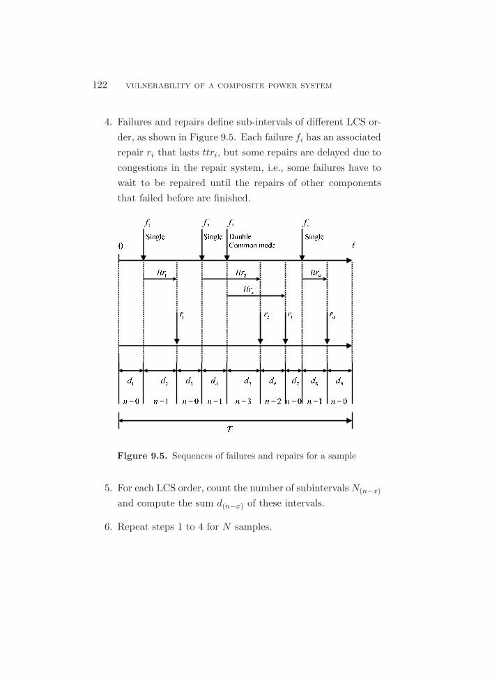
122 vulnerability of a composite power system
4. Failures and repairs define sub-intervals of different LCS or-
der, as shown in Figure 9.5. Each failure fi has an associated
repair ri that lasts ttri, but some repairs are delayed due to
congestions in the repair system, i.e., some failures have to
wait to be repaired until the repairs of other components
that failed before are finished.
��������������� � ��
�
�� �� ����� �� ��� ���� − �� −
�� − �� − �� − �� −�� − �� −
�� −
�� � !" # $%&'() $%&'()$%&'() *+,-().+//+& /+0)
Figure 9.5. Sequences of failures and repairs for a sample
5. For each LCS order, count the number of subintervals N(n−x)
and compute the sum d(n−x) of these intervals.
6. Repeat steps 1 to 4 for N samples.

examples 123
7. Compute for each sub-period k (month, semester, year, etc.)
of T the LCS indices in the following way:
Pn−x =
N∑
j=1
d(n−x)j
N ∗ T; (9.10)
Dn−x =
N∑
j=1
d(n−x)j
N∑
j=1
N(n−x)j
; (9.11)
Fn−x =
N∑
j=1
N(n−x)j
N ∗ T. (9.12)
Contrary to (9.5) and (9.9), the proposed method does not
require a table of possible LCS.
When using time-varying rates, (9.10)-(9.12) should not be
computed for a single sub-period equal to T , because variation is
lost; also, all SPP models have to be synchronized to a common
time reference.
9.6. Examples
The proposed method is applied to a study of LCS in the transmis-
sion zone of the one-area IEEE Reliability Test System (RTS) [7]
shown in Figure 9.6.
As pointed out by Billinton and Allan [4]:
“In many cases, severity associated with a contin-
gency event is inversely related to the frequency and
the probability of its occurrence. In other words, as the

124 vulnerability of a composite power system
Figure 9.6. The Single Area IEEE RTS
number of components involved in a simultaneous out-
age increases, both the probability and the frequency of
the contingency decrease.”
The analysis of results presented here thus focuses more on the
relative change in LCS indices than in their absolute magnitudes.

examples 125
9.6.1. Example 1: Constant Rates and Diverse Repair
Logistics
This example considers the following cases:
Case 1: Each component has a repair team dedicated to it.
Results are the same as those obtained when applying
(9.5)-(9.9). Failure and repair processes of all components
are modeled as HPP using RTS data.
Case 2: Three maintenance zones are considered; one for the
138 kV transmission lines, one for the power transform-
ers and one for the 230 kV transmission lines. The repair
service process in each maintenance zone follows the RTS
repair data.
Case 3: Similar to Case 2, but now three operating states are
considered for the power transformers, as shown in Fig-
ure 9.8. The nominal capacity (ONAF) state has failure
rate equivalent to 80% of the value given for the RTS and
a mean repair time of 768 hours (RTS data). The derated
capacity (ONAN) state has failure rate equivalent to 20%
the value given for the RTS and an assumed repair time
of 168 hours (one week).
Tables 9.1 to 9.3 show the results for T = 1 year and simula-
tions for 15 000 realizations. Relative changes in results (∆%) for
case 2 are computed with reference to case 1, and for case 3 are
computed with reference to case 2.
These results show that:
• For the system under study, LCS of order up to 4 are ex-
pected to occur.
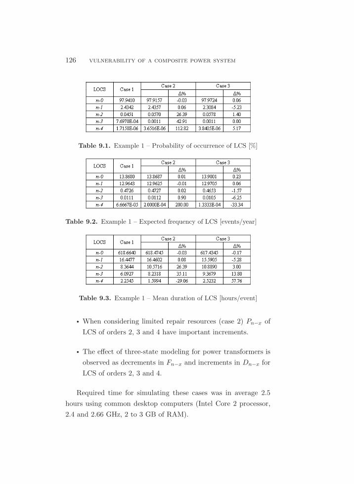
126 vulnerability of a composite power system
Table 9.1. Example 1 – Probability of occurrence of LCS [%]
Table 9.2. Example 1 – Expected frequency of LCS [events/year]
Table 9.3. Example 1 – Mean duration of LCS [hours/event]
• When considering limited repair resources (case 2) Pn−x of
LCS of orders 2, 3 and 4 have important increments.
• The effect of three-state modeling for power transformers is
observed as decrements in Fn−x and increments in Dn−x for
LCS of orders 2, 3 and 4.
Required time for simulating these cases was in average 2.5
hours using common desktop computers (Intel Core 2 processor,
2.4 and 2.66 GHz, 2 to 3 GB of RAM).

examples 127
9.6.2. Example 2: Increasing Failures Rates – Constant
Repair Rates
This example considers three maintenance zones with the same
repair models as in case 2 of example 1, but the failure rates are
now considered increasing functions of time, in order to represent
a situation of aging and lack of maintenance. Failure processes
are modeled using a PLP . The scale parameter λ is defined as
the permanent failure rate given as data for the RTS and a shape
parameter β = 1.5.
Tables 9.4 to 9.6 show results for year, two sub-periods per
year and simulations of 12 500 realizations. Relative changes (∆%)
in the indices are shown in Figures 9.7 to 9.9. These values are
computed with reference to the index value in the first sub-period
where it is non-zero. In Figure 9.7 results for LCS of order zero
cannot be seen due to its low magnitudes. In Figure 9.9 only
changes in mean duration for LCS of order zero, one and two are
presented; results for LCS of orders 3 and 4 are not presented
because they show high oscillation.
Table 9.4. Example 2 – Probability of occurrence of LCS [%]
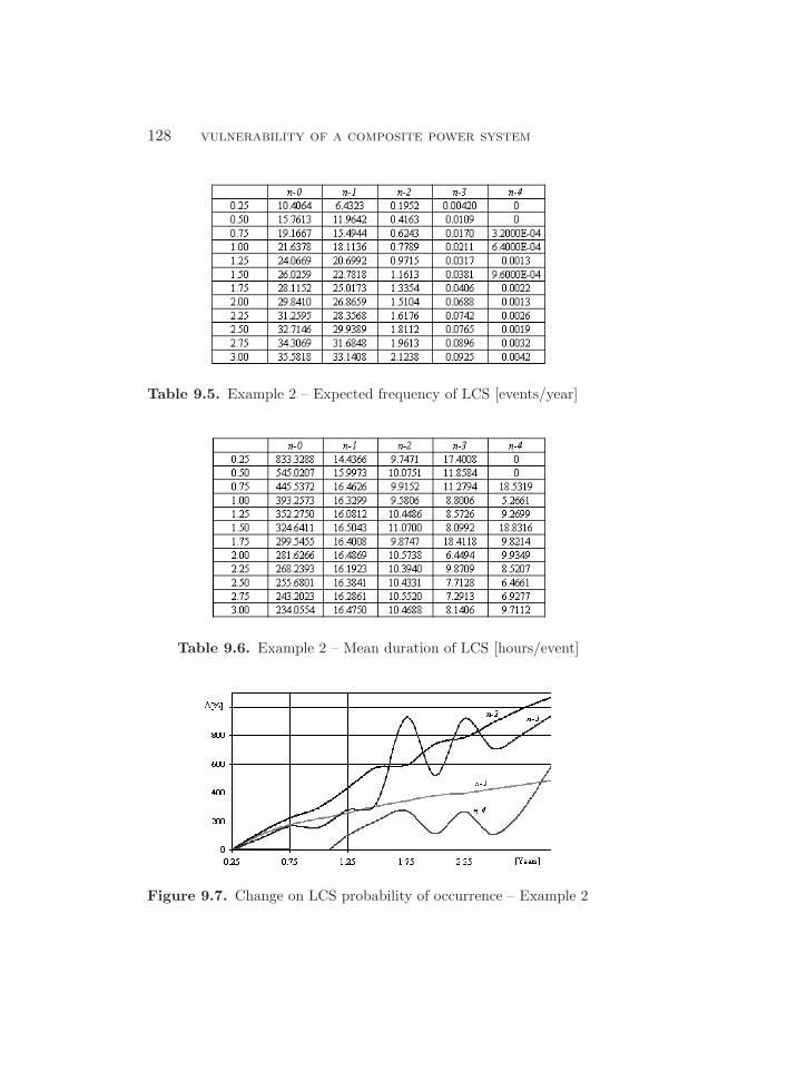
128 vulnerability of a composite power system
Table 9.5. Example 2 – Expected frequency of LCS [events/year]
Table 9.6. Example 2 – Mean duration of LCS [hours/event]
Figure 9.7. Change on LCS probability of occurrence – Example 2

examples 129
Figure 9.8. Change on LCS expected frequency – Example 2
Figure 9.9. Change on LCS mean duration – Example 2
These results show that:
• As time passes, Pn−x and Fn−x for LCS of orders 1 to 4 are
increasing functions of time. The increments in these indices
are huge.
• For the n − 0 operating state, Dn−x is the index that bet-
ter reflects the effect of increasing failure rates and constant
repair resources. It is a decreasing function of time.
Required time for simulating this case was in average 6.0 hours
using common desktop computers (Intel Core 2 processor, 2.4 and
2.66 GHz, 2 to 3 GB of RAM).
130 vulnerability of a composite power system
9.7. Conclusions
Due to the huge dimensions of the space of operating states of a
power system, a study of LCS is always a cumbersome task, no
matter what method is applied. The proposed method is a very
flexible modeling alternative but it requires significant computer
resources.
The presence of aging and other factors that produce increasing
component failure rates increases the risk of occurrence of high-
order loss of component scenarios. On the other hand, mainte-
nance strategies can decrease this risk. For this reason, it is nec-
essary an assessment method as the one proposed here, which can
manage time-varying rates.

Chapter 10
Main Conclusion
Vulnerability assessments of composite power systems have to in-
clude all those factors that can produce increasing component fail-
ure rates, such as aging and lack of resources for maintenance,
because they dramatically increase the risk that high-order loss of
component scenarios occur.
This also means that the vulnerability assessments must be
performed using methods than can manage time-varying rates.
To address this need, a method based on stochastic point process
modeling and a sequential Monte Carlo simulation is proposed in
this work.
131


References
[1] H. Ascher and H. Feingold. Repairable Systems Reliability:
Modeling, Inference, Misconceptions and Their Causes. Mar-
cel Dekker, 1984.
[2] H.E. Ascher and C.K. Hansen. Spurious exponentially ob-
served when incorrectly fitting a distribution to nonstationary
data. IEEE Transactions on Reliability, 47(4), Dec. 1998.
[3] N. Balijepalli, S. Venkata Subrahmanyan, and R.D. Christie.
Modeling and analysis of distribution reliability indices. IEEE
Transactions on Power Delivery, 19(4), Oct. 2004.
[4] R. Billinton and R.N. Allan. Reliability Assessment of Large
Electric Power Systems. Kluwer, 1988.
[5] C.A. Dortolina, J.J. Porta, and R. Nadira. An approach for
explicitly modeling the protective relaying system in substa-
tion reliability studies. IEEE Transactions on Power Systems,
6(4), 1991.
[6] T.F. Hassett, D.L. Dietrich, and F. Szidarovszky. Time-
varying failure rates in the availability & reliability analysis of
repairable systems. IEEE Transactions on Reliability, 44(1),
Mar. 1995.
133

134 references
[7] IEEE Task Force. The IEEE reliability test system - 1996.
IEEE Transactions on Power Systems, 14(3), Aug. 1999.
[8] IEEE Task Force. Vulnerability assessment for cascading fail-
ures in electric power systems. IEEE PES General Meeting,
2009.
[9] B. Klefsjo and U. Kumar. Goodness-of-fit tests for the power
law process based on the TTT plot. IEEE Transactions on
Reliability, 41(4), Dec. 1992.
[10] V.I. Kogan and R.J. Gursky. Transmission towers inventory.
IEEE Transactions on Power Delivery, 11(4), Oct. 1996.
[11] V.I. Kogan and T.L. Jones. An explanation for the decline in
URD cable failures and associated nonhomogeneous poisson
process. IEEE Transactions on Power Delivery, 9(1), Jan.
1994.
[12] M.T. Schilling, J.C.G. Praca, J.F. Queiroz, C. Singh, and
H. Ascher. Detection of ageing in the reliability analysis of
thermal generators. IEEE Transactions on Power Systems,
3(2), 1988.
[13] R.H. Stillman. Modeling failure data of overhead distribution
systems. IEEE Transactions on Power Delivery, 15(4), Oct.
2000.
[14] R.H. Stillman. Power line maintenance with minimal repair
and replacement. IEEE Annual Reliability and Maintainabil-
ity Symposium, 2003.
[15] W.A. Thomson. Point Processes Models with Applications to
Safety and Reliability. Chapman and Hall, 1988.

references 135
[16] J.F. Valencia. Confiabilidad de sistemas de proteccion de
transformadores de potencia del sistema CHEC [Reliability
of protective systems of power transformers of CHEC]. Grad-
uation Project, Universidad de los Andes, Bogota, 2009. (In
Spanish).
[17] C.J. Zapata. Analisis probabilıstico y simulacion [Proba-
bilistic analysis and simulation]. Universidad Tecnologica de
Pereira, 2010. (In Spanish).
[18] C.J. Zapata, A. Alzate, and M. Rıos. Reliability assessment of
substations using stochastic point processes and Monte Carlo
simulation. IEEE PES General Meeting, 2009.
[19] C.J. Zapata, C.M. Arbelaez, and C.A. Pulgarın. Indices de
confiabilidad de equipos de subestaciones de distribucion [Re-
liability indices of distribution substation equipment]. Mundo
electrico, 65, 2006. (In Spanish).
[20] C.J. Zapata, D.Y. Catano, and H.F. Suarez. Indices de confia-
bilidad de transformadores de distribucion [Reliability indices
of distribution transformers]. Mundo electrico, 57, 2004. (In
Spanish).
[21] C.J. Zapata and O.J. Hernandez. Indices de confiabilidad de
transformadores de potencia de subestacion de distribucion
[Reliability indices of distribution substation power trans-
formers]. Mundo electrico, 71, 2008. (In Spanish).
[22] C.J. Zapata, M.E. Leyes, and M.Y. Patino. Indices de con-
fiabilidad de circuitos primarios de distribucion [Reliability
indices of distribution feeders]. Mundo electrico, 69, 2007.
(In Spanish).
136 references
[23] C.J. Zapata and P.A. Montealegre. Problemas tecnicos en
la calidad del servicio de electricidad [Technical problems on
the quality of electricity service]. Mundo electrico, 68, 2007.
(In Spanish).
[24] C.J. Zapata and J.A. Ramırez. Indices de confiabilidad de
cortacircuitos en distribucion [Reliability indices of distribu-
tion cut-outs]. Mundo electrico, 66, 2007. (In Spanish).
[25] C.J. Zapata, S.C. Silva, O.L. Burbano, and J.A. Hernandez.
Repair models of power distribution components. IEEE
Transmission & Distribution Latin America Conference &
Exhibition, 2008.
[26] C.J. Zapata, S.C. Silva, H.I. Gonzalez, O.L. Burbano, and
J.A. Hernandez. Modeling the repair process of a power dis-
tribution system. IEEE Transmission & Distribution Latin
America Conference & Exhibition, 2008.
[27] C.J. Zapata, A. Torres, D.S. Kirschen, and M. Rıos. A
method for studying loss of component scenarios in a power
system using stochastic point processes. IEEE PES General
Meeting, 2009.
[28] C.J. Zapata, A. Torres, D.S. Kirschen, and M. Rıos. Reliabil-
ity assessment of protective schemes considering time varying
rates. International Review of Electrical Engineering, 4(6),
2009.
[29] C.J. Zapata, A. Torres, D.S. Kirschen, and M. Rıos. Some
misconceptions about the modeling of repairable components.
IEEE PES General Meeting, 2009.
[30] C.J. Zapata, A. Torres, D.S. Kirschen, and M. Rıos. Modeling
of protective system failures to operate for reliability studies

references 137
at the power system level using stochastic point processes.
International Review of Electrical Engineering, 5(2), 2010.