5SFOET JO JODPNF BOE DPOTVNQUJPO JOFRVBMJUZ JO … · cilios Argentina 1974,1980,1986-2010 Encuesta...

Trends in income and consumption inequality in Bolivia:A fairy tale of growing dwarfs and shrinking giants

Draft - Public disclosure unauthorized

Ahmed Eid1 Rodrigo Aguirre Werner L. Hernani-LimarinoFundación ARU

Abstract

This paper documents and describes the evolution of income and consumption inequality in Boliviabetween 1999 and 2011. We find that income and consumption inequality measured by the Gini in-dex both dropped 22% during the period we analyze, making Bolivia the top performer in the LatinAmerican region regarding income inequality reduction. To make a more complete description of thistrend, we make separate analysis for the urban an rural area. Changes in urban inequality are drivenby changes in the upper part of the distribution, as the 90-50 income and consumption percentile ra-tios fell 24%, as opposed to a 8% fall in the 50-10 ratio, for the subperiod 2005-2011. Changes in ruralinequality occur through the entire distribution in similar fashion, but are more intense before 2005,when the 90-50 and 50-10 ratios fell 30 and 26% respectively.

Keywords: Income, inequality, Consumption, inequality

1. Introduction

During many years, Bolivia has faced numerous challenges to reduce its poverty rates, and one of themost pressing concerns was the high levels of inequality its income distribution displayed ([29], [54],[25], [2], [41], [40], [31]). However, the 2000s marked the start of an inequality reduction trend in whichthe income Gini index fell 13 points, with a higher rate of decline in the last 6 years of the 1999-2011lapse: -3.4% against a -0.8% during 1999-2005. National consumption inequality followed a very sim-ilar pattern in terms of reduction rates and magnitude.

Nevertheless, this equalization process is not homogenous in time or by area. In the urban area,the decline started after 2005 with an annualized rate of income Gini reduction close to 4% (-3% forconsumption), while in the rural area the reduction occurred over twice as fast before 2005 in the caseof income, -2.28% pre-2005 against -1% between 2005 and 2011. The inequality decay for rural con-sumption is an unusual case of sustained reduction through the whole period af analysis, however ata much more modest rate of a little over 1% per year.

The objective of this paper is to provide a detailed description of the changes in the income andconsumption distributions at the national, urban and rural level, which ultimately led to the ob-served reductions in inequality. Additionally, the authors perform decomposition of commonly usedinequality indices to provide further insights on which component of income or consumption mayhave driven the decline, and to explore whether this reductions may be closing some gaps regardinginequality between groups. In this sense, this document only seeks to provide stylized facts of the re-duction process, not explanations regarding causes of the decline.

Preprint submitted to Elsevier July 18, 2013

Our results show pro-poor growth patterns of average income and consumption, in which the av-erage income for the bottom decile grew at rates comparable to the top performing economies in theworld, around 15% per year, while the average income for the top decile never grew over 5% per yearbetween 1999 and 2011. Comparing Brazil’s inequality reduction with Bolivia’s, makes our results evenmore puzzling: At similar GDP growth rates, Brazil Gini index fell 5 points in a similar lapse, even withmore efficient transfer policies ([37], [14], [38]). Finally, between group inequality is the componentwhich

The remainder of the document is organized as follows: section 3 explains the variable and datasetconstruction, section 4 describes national inequality trends and explains the distributional changesin urban and rural areas which led to the decline, section 5 shows the results for the index decomposi-tions, section 6 compares our results with the rest of the Latin American Region, and finally section 7conludes.

2. The Bolivian inequality decline in the literature: International trendaggregation and local lack of interest

Why is it now, in the second half of 2013, that the Bolivian case is being heard of? We believe thatthere are two main reasons behind this fact: A clear tendency to aggregate results at the regional level,neglecting the ever acknowledged heterogeneity in the region, and the second reason is that Bolivianeconomists do not appear to care about inequality anymore: The vast majority of the work on inequal-ity is conducted with data before 2005 with 2002 data, and after 2005 the research on inequality is veryscarce.

To begin the analysis of this issue, table 1 shows a summary of the latest available research on LatinAmerican inequality. 14 out of 17 of the reviewed documents were produced by economists affiliatedeither to the World Bank, CEDLAS or Tulane University, and 11 out of 17 use the SEDLAC databaseconstructed by CEDLAS and the World Bank. This inequality boom started on 2008, but its most pro-lific years are between 2009 and 2012. There is a broad consensus that labor income played the mostsignificant role in the inequality decline, and that the relevance of government transfers in this pro-cess varied by country. Argentina, Brazil and México are the cases most studied, but the rest of thecountries in the LAC region appear in 12 out of 17 studies. Most of the advertisement of the results ofthis research is done at a regional level, ignoring country-specific results. The inequality declines inBolivia, Venezuela and Ecuador are the most succesful, but they becomes hidden when looked froma regional perspective. Brazil, one of the most publicized cases of inequality reduction, doesn’t evenrank among the countries with the highest decline.

Regarding the Bolivian literature on inequality, most of it was done before 2005 from a variety ofperspectives: fiscal policy, natural resources and labor market. This may have been driven by the highlevels of inequality recorded during those years. But when inequality started falling after 2005, only acouple of studies recorded the decline, but failed to grasp the magnitude of their findings and to directthe attention towards the relevance of the decline in the Latin american context. As a matter of fact,none of the local studies is even concerned with the extent or speed of the decline, these research isconcerned with how other variables or policies affect inequality, a necesary step once the distribu-tional changes have been accounted for.

2

Table 1: Most recent literature on Latin American inequality

Author Title Year Countries Studied Data Source Period of Analysis

Alejo J., Bergolo M., Carbajal F. Las Transferencias Públicas y su impactodistributivo: La Experiencia de los Paísesdel Cono Sur en la década de 2000

2013 Argentina,Brasil,Chile and Uruguay National Household Surveys 2000-2005,2005-2009,2000-2009

Azevedo J. Decomposing the Recent Inequality De-cline in Latin America

2012 Argentina,Brazil,Chile,Colombia,Costa Rica,Dominican Rep., Ecuador,El Salvador, Hon-duras,Mexico,Panama,Paraguay,Peru,Uruguay

SEDLAC 2000-2010

Azevedo J., Davalos M., Diaz-Bonilla C.,Atuesta B., Castaneda R.

Fifteen Years of Inequality in Latin Amer-ica How Have Labor Markets Helped?

2013 Argentina,Brazil,Bolivia,Chile,Colombia,Costa Rica,Dominican Republic,Ecuador,El Sal-vador,Honduras,Mexico,Panama,Paraguay,Peru,Uruguay

SEDLAC 1995-2000,2000-2005,2005-2010

Cornia G. Inequality Trends and their Determi-nants: Latin America over 1990-2010

2012 Argentina,Peru,Ecuador,Paraguay,Brazil,Panama,Venezuela,El Sal-vador,Chile,Bolivia,Honduras,Mexico,Guatemala,Dominican Republic,Uruguay,CostaRica,Nicaragua,Colombia

SEDLAC 1990-2002,2002-2009

De Ferranti D, Perry G., Ferreira F., WaltonM., Coady D., Cunnigham W., GaspariniL., Jacobsen J., Matsuda Y., Robinson J.,Sokoloff K., Wodon Q.

Inequality in Latin America: Breakingwith History?

2003 Argentina,Brazil,Bolivia,Chile,Colombia,Costa Rica,Dominican Republic,Ecuador,El Sal-vador,Honduras,Mexico,Panama,Paraguay,Peru,Uruguay

Household surveys 1990-2001

Gasparini L. Income Inequality in Latin America andthe Caribbean: Evidence from HouseholdSurveys

2003 Argentina,Bolivia,Brazil,Chile,Colombia,Costa Rica,Ecuador,El Sal-vador,Guatemala,Honduras,Jamaica,Mexico,Nicaragua,Panama,Paraguay,Peru,DominicanRepublic,Trinidad and Tobago,Uruguay,Venezuela.

52 household surveys 1989-2001

Gasparini L., Lustig N. The Rise and Fall of Income Inequality inLatin America

2011 Argentina, Brazil, Mexico PNAD, ENIGH, EPH 1974-2006, 1981-2006

Gasparini L., Cruces G., Tornarolli L. Recent trends in income inequality inLatin America

2009 Argentina,Chile,Brazil,Uruguay,Paraguay,Bolivia,Peru,Ecuador,Colombia,CostaRica,Panama,Mexico,Venezuela,Nicaragua,Guatemala,El Salvador,Dominican Repub-lic,Honduras

SEDLAC 1992-2006

Gasparini L., Cruces G., Tornarolli L. Mar-chionni M.

A Turning Point? Recent Developmentson Inequality in Latin America and theCaribbean

2009 Argentina,Chile,Brazil,Uruguay,Paraguay,Bolivia,Peru,Ecuador,Colombia,CostaRica,Panama,Mexico,Venezuela,Nicaragua,Guatemala,El Salvador,Dominican Repub-lic,Honduras

SEDLAC 1990-2006

Goñi E., Lopez J.,Serven L. Fiscal Redistribution and Income In-equality in Latin America

2008 Argentina,Brazil,Chile,Colombia,Mexico,Peru Data on transfers and taxes 2006

Lopez-Calva L., Lustig N. The recent decline of inequality in Lati-nAmerica: Argentina, Brazil, Mexico andPeru

2009 Argentina,Brazil,Mexico and Peru SEDLAC 2000-2006

Lustig N. Taxes, Transfers, and Income Redistribu-tion in Latin America

2012 Argentina,Bolivia,Brazil,Mexico,Peru,Uruguay SEDLAC 2012

Lustig N., Lopez-Calva L., Ortiz-Juarez E. The decline in inequality in Latin Amer-ica: How much, since when and why

2011 Argentina,Peru,Paraguay,El Salvador,Brazil,Panama,Mexico,Venezuela,Chile,DominicanRepublic,Bolivia

SEDLAC 1990-2000,2000-2009

Lustig N., Lopez-Calva L., Ortiz-Juarez E. Declining Inequality in Latin America inthe 2000s: The Cases of Argentina, Brazil,and Mexico

2012 Argentina,Brazil and Mexico SEDLAC 1990-2010

Medina F., Galvan M. Descomposición del coeficiente de Ginipor fuentes de ingreso: Evidencia em-pírica para América Latina 1999-2005

2008 Argentina,Bolivia,Brazil,Chile,Colombia,Costa Rica,Ecuador,El Sal-vador,Guatemala,Honduras,Mexico,Nicaragua,Panama,Paraguay,Dominican Repub-lic,Uruguay,Venezuela.

National Household Surveys 1999-2005

World Bank Global Trends in Income Inequality 2012 18 LAC countries SEDLAC 2001-2009World Bank Fifteen Years of Inequality Reduction in

Latin America2011 Argentina,Bolivia,Brazil,Chile,Colombia,Costa Rica,El Salvador,Honduras,Mexico,Panama,Paraguay,Peru,

Dominican Republic,Uruguay.SEDLAC 1995-2000,2000-2009,1995-2009

Source: Authors’ elaboration

Table 2: Most recent literature on Bolivian inequality

Author Title Years of data used

Official literature

INE,UDAPE Estimación del gasto de consumo combinando el Censo 2001 y las Encuestas de hogares 1999-2001Jiménez W., Lizárraga S. Ingresos y Desigualdad en Área Rural de Bolivia 1999-2001Yanez E., 2004 Qué explica la desigualdad en la distribución del ingreso en las áreas urbanas de bolivia: un análisis

a partir de un modelo de microsimulación1999-2002

Landa F., 2004 ¿Las dotaciones de la población ocupada son la única fuente que explican la desigualdad de ingre-sos en bolivia? una aplicación de las microsimulaciones

1989-1999

Independent literature

Gutierrez C., 2008 Analysis of Poverty and Inequality in Bolivia, 1999-2005: A Microsimulation Approach 1999-2005Vargas,J.F., 2012 Declining Inequality in Bolivia: How and Why 2003/2004,2005,2008,2009Villegas H., 2006 Desigualdad en el Area Rural de Bolivia: Cuan Importante es la educacion? 1999-2002Andersen L., Faris R. Natural Gas and Inequality in Bolivia 1999Nina O. El Impacto Distributivo de la Política Fiscal en Bolivia 2003-2004Muriel B. Rethinking Earnings Determinants in the Urban Areas of Bolivia 2003-2004Jspatz J.,Steneir S. Post-Reform Trends in Wage Inequality: The Case of Urban Bolivia 19891997Yanez E. El Impacto del Bono Juancito Pinto. Un Análisis a Partir de Microsimulaciones 2005Gasparini L.,Marchionni M., Gutierrez F. Simulating Income Distribution Changes in Bolivia:a Microeconometric Approach 1993-2002Lay J., Thiele R., Wiebelt M. Resource Booms, Inequality and Poverty: The Case of Gas in Bolivia 2001Andersen L., Caro J., Faris R., Medinacelli M. Natural Gas and Inequality in Bolivia After Nationalization 1997

Source: Authors’ elaboration

Public data availability, shown on table 3, may explain why the Bolivian case didn’t receive theattention it could have gotten. While Brazil, Mexico and Argentina have data available until the late2000s, Bolivian data is only available until 2007 in the SEDLAC. However, Bolivian household surveyswere conducted in 2008, 2009, 2011 and 2012. This means that there are 4 years of collected datawaiting to be analyzed. Household survey designs changes occur frequently in Bolivia, so a one-size-fits-all harmonization process may not be the most suitable to solve the problem of changing surveydesign.

3

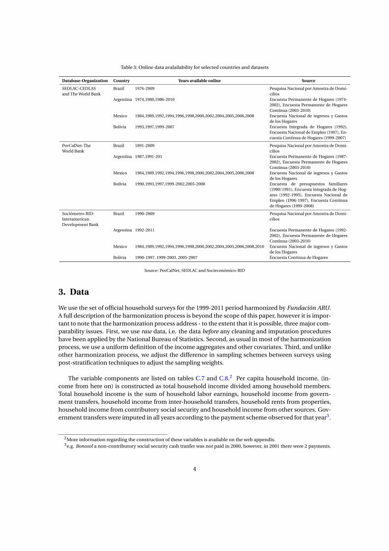
Table 3: Online data avalailability for selected countries and datasets

Database-Organization Country Years available online Source

SEDLAC-CEDLASand The World Bank

Brazil 1976-2009 Pesquisa Nacional por Amostra de Domi-cilios

Argentina 1974,1980,1986-2010 Encuesta Permanente de Hogares (1974-2002), Encuesta Permanente de HogaresContinua (2003-2010)

Mexico 1984,1989,1992,1994,1996,1998,2000,2002,2004,2005,2006,2008 Encuesta Nacional de ingresos y Gastosde los Hogares

Bolivia 1993,1997,1999-2007 Encuesta Integrada de Hogares (1992),Encuesta Nacional de Empleo (1997), En-cuesta Continua de Hogares (1999-2007)

PovCalNet-TheWorld Bank


Argentina 1987,1991-201 Encuesta Permanente de Hogares (1987-2002), Encuesta Permanente de HogaresContinua (2003-2010)

Mexico 1984,1989,1992,1994,1996,1998,2000,2002,2004,2005,2006,2008 Encuesta Nacional de ingresos y Gastosde los Hogares

Bolivia 1990,1993,1997,1999-2002,2005-2008 Encuesta de presupuestos familiares(1990/1991), Encuesta Integrada de Hog-ares (1992-1995), Encuesta Nacional deEmpleo (1996-1997), Encuesta Continuade Hogares (1999-2008)

Sociómetro-BID-InteramericanDevelopment Bank


Argentina 1992-2011 Encuesta Permanente de Hogares (1992-2002), Encuesta Permanente de HogaresContinua (2003-2010)

Mexico 1984,1989,1992,1994,1996,1998,2000,2002,2004,2005,2006,2008,2010 Encuesta Nacional de ingresos y Gastosde los Hogares

Bolivia 1990-1997, 1999-2003, 2005-2007 Encuesta Continua de Hogares

Source: PovCalNet, SEDLAC and Socieconómico-BID

3. Data

We use the set of official household surveys for the 1999-2011 period harmonized by Fundación ARU.A full description of the harmonization process is beyond the scope of this paper, however it is impor-tant to note that the harmonization process address - to the extent that it is possible, three major com-parability issues. First, we use raw data, i.e. the data before any cleaning and imputation procedureshave been applied by the National Bureau of Statistics. Second, as usual in most of the harmonizationprocess, we use a uniform definition of the income aggregates and other covariates. Third, and unlikeother harmonization process, we adjust the difference in sampling schemes between surveys usingpost-stratification techniques to adjust the sampling weights.

The variable components are listed on tables C.7 and C.8.2 Per capita household income, (in-come from here on) is constructed as total household income divided among household members.Total household income is the sum of household labor earnings, household income from govern-ment transfers, household income from inter-household transfers, household rents from properties,household income from contributory social security and household income from other sources. Gov-ernment transfers were imputed in all years according to the payment scheme observed for that year3.

2More information regarding the construction of these variables is available on the web appendix.3e.g. Bonosol a non-contributory social security cash tranfer was not paid in 2000, however, in 2001 there were 2 payments.

4

Per capita household consumption (consumption from this point on) is constructed in an iden-tical fashion. It’s components are food, non-food, housing, utilities, durable goods, health and edu-cation expenditures. Education expenditure was imputed for the year 2002 using data from 2001. Weestimate the percentiles of total household expenditure for both years, and then impute the percentileaverage from 2001 to all households in that percentile in 2002.

Our working datasets are free of missing values and outliers. We treat each welfare measure sep-arately when it comes to construct a working dataset, i.e. households which were dropped from theincome sample may be present in the consumption sample and viceversa, so we have different in-come and consumption samples. Additionally, we treat each region by itself when dropping missingincomes and outliers: this results in an urban sample free of missing values and outliers, and a ru-ral sample with the same features. To obtain the national sample, we append the urban and ruraldatasets.

The first step we took was to drop from the sample all households with missing per capita house-hold income or consumption components. Then we use the Blocked Adaptive Computationally-efficient Outlier Nomination (BACON) algorithm to nominate and drop outliers in the sample. Theuse of this algorithm requires the researcher to provide a subset of the data for which he is sure thereare no outliers, and then the algorithm starts to look for unusually large observations in the remainingsubset which may or may not contain outliers, using a Mahalanobis distance and then performing a¬2 test to determine whether an observation is an outlier. We used Æ = 0.0001. For every estimationand description from this point on, we will be using this sample. 4

4. Trends in Bolivian income and consumption inequality

Figure 1 shows the evolution of Bolivian income and consumption inequality, measured by the Giniindex, from 1999 to 2011. National income inequality fell 13 Gini points (.59 to .46) in this 13 yearperiod, while national consumption inequality dropped from 0.47 to 0.37 in the same lapse. As re-markable those figures are by themselves, they become even more surprising when we take 2005 asreference point: Until that year, national income inequality fell only 3 Gini points, and national con-sumption inequality fell only 2. This leaves us with a 17.85% reduction in national income inequalityand a 17.78% in national consumption inequality in 6 years.

We imputed those payments in 2001.4Descriptions and estimations based on the full, P(0.001) and P(0.0001) samples are available in the web appendix

5

Figure 1: Gini index evolution by outcome

.35

.4

.45

.5

.55

.6

.65

.7

Gin

i ind

ex

1999 2001 2003 2005 2007 2009 2011Year

National Urban Rural

Per capita household income

.35

.4

.45

.5

.55

.6

.65

.7

Gin

i ind

ex

1999 2001 2003 2005 2007 2009 2011Year

National Urban Rural

Per capita household consumption

Source: Author’s estimation based on Fundación ARU’s harmonized series of household surveys. Zeros and outliers were droppped from the sam-ple. Outliers were nominated using the BACON algorithm with Æ = 0.0001. Per capita household income (consumption) equals total householdincome (consumption) divided among household members. Total household income is the sum of labor and social security income, govern-ment (imputed) and inter-household transfers, rents from properties and other sources. Total consumption is the sum of food, non-food, health,education, durable goods, utilities and housing expenditures. Hedonic regressions by type of house were used to estimate and impute housingexpenditure.

However, inequality did not display the same behavior when the analysis is split by area: Urbanincome inequality behaved erratically until 2005, and rose from 0.49 to 0.51. It all became downhillsince then, to reach a 0.40 value in 2011. Urban consumption inequality shows a smoother trend, butalso displays a 2 point rise during 1999-2005, from .38 to .40. After 2005, the biggest fall is seen from2005 to 2006, to a level of .37 which remains unchanged until 2009. Finally, it goes down to its lowestlevel in 2011: 0.35, which makes a total fall of 7 points in 6 years.

Rural income inequality fell from 0.64 to 0.54 in 1999-2003, then rose to 0.61 in 2006, and thenstarted to fall again, finally reaching a level of 0.53 in 2011. Consumption inequality in the rural areadidn’t fall as much when compared to income or urban trends, however it fell from 0.43 to 0.40 in1999-2005 and to an all-period low of 0.38 in 2011. This disparities in trends by area and period areour motivation to conduct separate analysis for each area.

Changes in an income or consumption distribution may be driven by changes above or below themedian: Inequality may fall because those in the lower part are catching up with those in a higherposition in the distribution, or because incomes in the upper tail are falling to levels closer to those inlower relative positions. To distinguish between changes in the lower or upper tail, we also documentthe evolution of the 50-10 and 90-50 percentile ratios, displayed on figure 2.

6

Figure 2: Percentile ratios evolution by outcome

2

2.5

3

3.5

4

Perc

entil

e ra

tio

1999 2001 2003 2005 2007 2009 2011Year

90-50 50-10

Income

2

2.5

3

3.5

4

Perc

entil

e ra

tio

1999 2001 2003 2005 2007 2009 2011Year

90-50 50-10

Consumption

Urban Bolivia

2

4

6

8

10

Perc

entil

e ra

tio

1999 2001 2003 2005 2007 2009 2011Year

90-50 50-10

Income

2

4

6

8

10Pe

rcen

tile

ratio

1999 2001 2003 2005 2007 2009 2011Year

90-50 50-10

Consumption

Rural Bolivia


Looking first at the urban income ratios, reveals that most of the decline in inequality came fromchanges in the top of the distribution: the 90-50 ratio fell from 3.45 to 2.6 during 2005-2011, after notdisplaying abrupt changes during 1999-2006. The 50-10 ratio fell slightly in 1999-2011, from 3.04 to2.51. The trend for urban consumption percentile ratios is similar: the 90-50 fell from 2.63 to 2.52 un-til 2005, and then started a downhill tendency until 2.17 in 2011. The 50-10 urban consumption ratiorose from 2.12 to 2.32 in 1999-2005, and fell to 2.02 in 2011.

Turning to rural income ratios, the rate of decline after 2005 is very similar for the two ratios con-sidered, they dropped at yearly rates of -1.63%(90-50) and -1.80%(50-10). The only noticeably largerdecline is seen before 2005, period in which the 50-10 ratio fell from 7.2 to 5.36 and the 90-50 ratio didso from 5.41 to 3.77. For rural consumption the scenario shows trends with very little change, as the50-10 ratio remained constant at 2.70 and the 90-50 fell slightly from 2.86 to 2.51 until 2005. During2005-2011, there are relatively small declines in both indicators, the 90-50 ratio dropped until 2.29 andthe 50-10 fell until 2.59.

7

Yearly growth rateIncome Consumption

1999-2011Gini 90-10 90-50 50-10 Gini 90-10 90-50 50-10

National -2.09 -10.83 -3.09 -7.98 -2.03 -5.58 -2.36 -3.30Urban -1.68 -3.67 -2.12 -1.59 -1.23 -1.80 -1.62 -0.19Rural -1.63 -6.96 -3.77 -3.31 -1.17 -2.16 -1.82 -0.34

1999-2005National -0.80 -12.75 -1.50 -11.42 -0.62 -5.95 -1.46 -4.56Urban 0.58 -1.23 0.40 -1.62 0.52 0.82 -0.72 1.55Rural -2.28 -10.39 -5.87 -4.81 -1.11 -2.16 -2.17 0.01

2005-2011National -3.37 -8.87 -4.66 -4.41 -3.41 -5.22 -3.25 -2.03Urban -3.88 -6.05 -4.57 -1.55 -2.95 -4.35 -2.50 -1.90Rural -0.99 -3.40 -1.63 -1.80 -1.23 -2.15 -1.47 -0.69

Total variationIncome Consumption

Gini 90-10 90-50 50-10 Gini 90-10 90-50 50-101999-2011

National -22.4 -74.73 -31.41 -63.15 -21.79 -49.82 -24.91 -33.17Urban -18.38 -36.15 -22.64 -17.46 -13.82 -19.59 -17.75 -2.23Rural -17.93 -57.93 -36.96 -33.26 -13.18 -23.01 -19.78 -4.03

1999-2005National -4.68 -55.88 -8.68 -51.69 -3.68 -30.79 -8.42 -24.43Urban 3.51 -7.141 2.44 -9.35 3.17 4.99 -4.26 9.66Rural -12.9 -48.23 -30.42 -25.6 -6.47 -12.27 -12.31 0.04

2005-2011National -18.59 -42.71 -24.9 -23.72 -18.8 -27.49 -18.01 -11.57Urban -21.15 -31.24 -24.49 -8.94 -16.46 -23.41 -14.09 -10.85Rural -5.78 -18.73 -9.39 -10.3 -7.18 -12.23 -8.51 -4.07


Looking at total variations in the lower panel of table 4, it is clear that rural income inequality fallsduring the 13 years of analysis, but the fall is faster between 1999 and 2005. The decline in urban in-equality occurs after 2005, before this year it rose 3.5% (Gini index). Urban consumption inequalityfalls mostly through changes above the median, since the 90-50 ratio fell before and after 2005, unlikethe 50-10 ratio that rose almost 10% between 1999 and 2005. Rural consumption inequality also felldriven by changes in the upper tail - -12% in 1999-2005 and -8.5% in 2005-2011.

4.1. Urban inequality

Let us look closer at the distributional changes in the urban income and consumption distributions.Figure 3 shows the yearly growth rate for the average income and consumption by percentile.

8

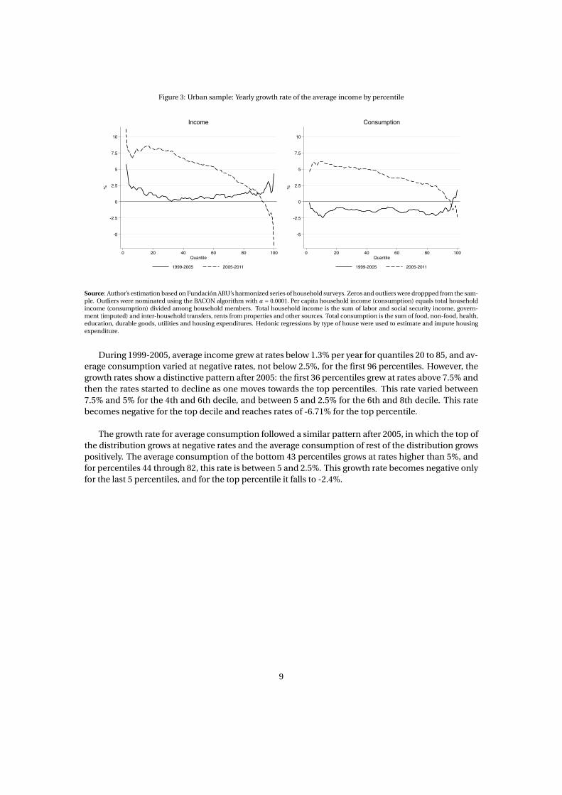
Figure 3: Urban sample: Yearly growth rate of the average income by percentile

-5

-2.5

0

2.5

5

7.5

10

%

0 20 40 60 80 100Quantile

1999-2005 2005-2011

Income

-5

-2.5

0

2.5

5

7.5

10

%

0 20 40 60 80 100Quantile

1999-2005 2005-2011

Consumption


During 1999-2005, average income grew at rates below 1.3% per year for quantiles 20 to 85, and av-erage consumption varied at negative rates, not below 2.5%, for the first 96 percentiles. However, thegrowth rates show a distinctive pattern after 2005: the first 36 percentiles grew at rates above 7.5% andthen the rates started to decline as one moves towards the top percentiles. This rate varied between7.5% and 5% for the 4th and 6th decile, and between 5 and 2.5% for the 6th and 8th decile. This ratebecomes negative for the top decile and reaches rates of -6.71% for the top percentile.

The growth rate for average consumption followed a similar pattern after 2005, in which the top ofthe distribution grows at negative rates and the average consumption of rest of the distribution growspositively. The average consumption of the bottom 43 percentiles grows at rates higher than 5%, andfor percentiles 44 through 82, this rate is between 5 and 2.5%. This growth rate becomes negative onlyfor the last 5 percentiles, and for the top percentile it falls to -2.4%.

9

Figure 4: Urban sample: Income and consumption Lorenz curves

0

.1

.2

.3

.4

.5

.6

.7

.8

.9

1L(p)

0 10 20 30 40 50 60 70 80 90 100Percentile

1999 2005 2011

0

.1

.2

.3

.4

.5

.6

.7

.8

.9

1

L(p)

0 10 20 30 40 50 60 70 80 90 100Percentile

1999 2005 2011


This differential in growth rates for average income and consumption is inevitably reflected inchanges in income and consumption shares by quantile. The top figures in figure 4 show the incomeand consumption Lorenz curves for 1999, 2005 and 2011. In 1999, the first half of the income distribu-tion held 18% of total income, and in 2011 this share grew to 23%. Regarding urban consumption, the2011 curves also dominates the other 2, but the change is smaller than the one observed for income.

10

Figure 5: Urban sample: Evolution of income and consumption shares

0

10

20

30

40

50

60

70

80

90

100

%

1999

2000

2001

2002

2003

2004

2005

2006

2007

2008

2009

2011

Income shares by decile

1 2 3 4 5 6 7 8 9 10

0

10

20

30

40

50

60

70

80

90

100

%

1999

2000

2001

2002

2005

2006

2007

2008

2009

2011

Consumption shares by decile

1 2 3 4 5 6 7 8 9 10

2

4

6

8

10

12

%

1999 2001 2003 2005 2007 2009 2011Year

96 97 98 99 100

Income shares for the top 5 percentiles

2

4

6

8

10

12

%

1999 2001 2003 2005 2007 2009 2011Year

96 97 98 99 100

Consumption shares for the top 5 percentiles


To look at distributional changes from a different perspective, figure 8 shows the evolution of in-come and consumption shares by decile. figure 8 gives a better view on the dramatic losses in incomeshare, suffered by the top decile, which held 40% of total income in 1999 and 2005, but in 2011 thisshare dropped to 30%. In the bottom panel, it is clear that the largest portion of the income share lossoccurred in the top percentile, whose share was cut in nearly half during 2005-2011 (11% to 6%).

Changes in urban consumption shares were more modest: the share of the bottom half grew from24% in 1999 to 28% in 2011.The losses for the consumption top decile were also smaller than the lossesof the income top decile, from a 30% in 1999 and 2005, it fell to 26% in 2011. The top percentile wasalso the biggest loser, but its share was cut from nearly 7 to 5%.

4.2. Rural inequality

The distributional changes that occurred in the rural area between 1999 and 2011 are not the samethan those for the urban area. As figure 6 shows, average income growth was positive for the entiredistribution, and was not close to zero before 2005, in fact, that is the period with higher growth ratesfor the first 64 percentiles. The average income for the top percentiles grew through the entire 13 year

11

lapse, but at a smaller rate than the average income of lower income tail, which grew over 20% forsome percentiles.

Figure 6: Rural sample: Yearly growth rate of the average income by percentile

-5

0

5

10

15

20

%

0 20 40 60 80 100Quantile

1999-2005 2005-2011

Income

-5

0

5

10

15

20

%0 20 40 60 80 100

Quantile

1999-2005 2005-2011

Consumption


The growth rates for average consumption were also positive before and after 2005, and the differ-ence between growth rates for the top and bottom percentiles is almost non-existant: During 1999-2005, the growth speed of the average consumption never surpassed 5%, and was never negative. After2005, it fluctuated around 10% for the first 95 percentiles of the distribution, the top 5 quantiles grewat a rate of 5%.

12

Figure 7: Rural sample: Income and consumption shares by quantile

0

.1

.2

.3

.4

.5

.6

.7

.8

.9

1L(p)

0 10 20 30 40 50 60 70 80 90 100Percentile

1999 2005 2011

0

.1

.2

.3

.4

.5

.6

.7

.8

.9

1

L(p)

0 10 20 30 40 50 60 70 80 90 100Percentile

1999 2005 2011


The 2011 Lorenz curves dominate the 1999 and 2005 curves, for both income and consumption.In the case of income, the bottom five deciles held only 8.76% of total income, in 2005 this share grewto 13.28% and then in 2011, it reached its peak level of 15.18%. Unlike the urban top income decilewhich decreased its income share in 25% during 2005-2011, the share of the top rural income decilefell from 50 to 40% during 1999-2005, and in 2011 this percentage remained constant. The changesin rural consumption shares are also minimal: the top consumption share fluctuated between 32%and 29% throughout 1999-2011, but the bottom half had its share modestly increased: from 21% in1999 to 24% in 2011. As in the case for urban indicators, the top income and consumption percentileswere the ones with largest share losses: from 12% to 9% in the case of income, and from 6.5% to 5% inconsumption, both during 2005-2011.

13

Figure 8: Rural sample: Evolution of income and consumption shares

0

10

20

30

40

50

60

70

80

90

100

%

1999

2000

2001

2002

2003

2004

2005

2006

2007

2008

2009

2011

Income shares by decile

1 2 3 4 5 6 7 8 9 10

0

10

20

30

40

50

60

70

80

90

100

%

1999

2000

2001

2002

2005

2006

2007

2008

2009

2011

Consumption shares by decile

1 2 3 4 5 6 7 8 9 10

0

3

6

9

12

15

18

%

1999 2001 2003 2005 2007 2009 2011Year

96 97 98 99 100

Income shares for the top 5 percentiles

0

3

6

9

12

15

18

%

1999 2001 2003 2005 2007 2009 2011Year

96 97 98 99 100

Consumption shares for the top 5 percentiles


5. Decomposing the trends in inequality

To shed light on the structure of inequality in Bolivia, we perform 2 widely used decompositions: a by-group decomposition of inequality, and a decomposition by outcome component. These sets of de-compositions are not available for every inequality measure: To perform a by-group decomposition,an inequality measure must be additively decomposable. [12] proves that all the measures belongingto the Generalized Entropy family satisfy such property, hence we perforn this decomposition on 3measures of that family, the mean log deviation (GE(0)), the Theil index (GE(1)) and half the square ofthe coefficient of variation (GE(2)).

To conduct decompositions by income component, we follow two approaches. The first is the ap-proach proposed by [43] in which the GE(2) measure is decomposed. To continue our analysis basedon the Gini index, we also perform the decomposition proposed by Lerman and Yitzhaki who decom-pose the Gini index by income source. The methods and results for these exercises are explained inthe followong subsections.

14

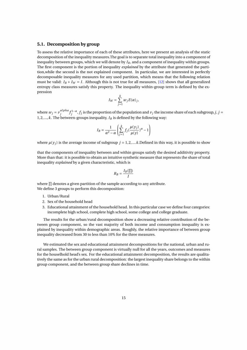
5.1. Decomposition by group

To assess the relative importance of each of these attributes, here we present an analysis of the staticdecomposition of the inequality measures.The goal is to separate total inequality into a component ofinequality between groups, which we will denote by I

B

, and a component of inequality within groups.The first component is the portion of inequality explained by the attribute that generated the parti-tion,while the second is the not explained component. In particular, we are interested in perfectlydecomposable inequality measures for any used partition, which means that the following relationmust be valid: I

B

+ I

W

= I . Although this is not true for all measures, [12] shows that all generalizedentropy class measures satisfy this property. The inequality within-group term is defined by the ex-pression

I

W

=kX

j=1w

j

E(Æ)j

,

where w

j

= v

al pha

j

f

1°Æj

, f

j

is the proportion of the population and v

j

the income share of each subgroup, j , j =1,2, ...,k. The between-groups inequality, I

B

is defined by the following way:

I

B

= 1Æ2 °Æ

√kX

j=1f

j

(µ(y

j

)

µ(y))Æ°1

!

where µ(y

j

) is the average income of subgroup j = 1,2, ....k.Defined in this way, it is possible to show

that the components of inequality between and within groups satisfy the desired additivity property.More than that: it is possible to obtain an intuitive synthetic measure that represents the share of totalinequality explained by a given characteristic, which is

R

B

= I

B

(Q

)I

whereQ

denotes a given partition of the sample according to any attribute.We define 3 groups to perform this decomposition:

1. Urban/Rural2. Sex of the household head3. Educational attainment of the household head. In this particular case we define four categories:

incomplete high school, complete high school, some college and college graduate.

The results for the urban/rural decomposition show a decreasing relative contribution of the be-tween group component, so the vast majority of both income and consumption inequality is ex-plained by inequality within demographic areas. Roughly, the relative importance of between groupinequality decreased from 30 to less than 10% for the three measures.

We estimated the sex and educational attainment decompositions for the national, urban and ru-ral samples. The between group component is virtually null for all the years, outcomes and measuresfor the houselhold head’s sex. For the educational attainment decomposition, the results are qualita-tively the same as for the urban rural decomposition: the largest inequality share belongs to the withingroup component, and the between group share declines in time.

15

Table 4: Decomposition of generalized enthropy measures by demographic area

Income Consumption

GE(0) GE(1) GE(2) GE(0) GE(1) GE(2)

W

g

B

g

W

g

B

g

W

g

B

g

W

g

B

g

W

g

B

g

W

g

B

g

1999 .616 .208 .505 .16 1.124 .135 .275 .135 .267 .113 .416 .12000 .709 .201 .622 .157 1.622 .134 .305 .144 .319 .12 .565 .1052001 .579 .14 .522 .115 1.109 .101 .285 .118 .302 .1 .507 .0892002 .634 .167 .604 .133 1.523 .114 .306 .1 .332 .086 .575 .0782003 .51 .116 .527 .098 1.161 .0872004 .471 .114 .48 .096 1.007 .0852005 .528 .116 .529 .097 1.21 .085 .269 .094 .285 .081 .476 .0722006 .533 .12 .476 .1 .952 .087 .259 .082 .254 .071 .368 .0642007 .491 .086 .437 .074 .795 .066 .222 .062 .228 .055 .35 .0512008 .46 .073 .453 .064 .953 .058 .22 .054 .218 .048 .301 .0442009 .434 .084 .397 .072 .753 .064 .213 .042 .215 .039 .299 .0362011 .374 .043 .336 .039 .501 .036 .203 .033 .201 .03 .268 .028

5.2. Decompositions by income source

In order to decompose income inequality into the various sources of income, we use the methodologyof [46]. This has the advantages of being invariant to choice of inequality measure and allowing fora simple decomposition of changes.By definition, each individual’s income can be broken down intothe sum of income received from different sources, i.e.

Y

i

=X

Y

f

i

where Y

f

i

is the income individual i receives from income source f . The idea behind the incomesource decomposition is that we can similarly break down total income inequality into the part thateach income source is responsible for. The component inequality weight of factor f , s

f

(y), is then thecovariance of this factor with total income, scaled by the total variance of income, i.e.

s

f

(y) = cov[Y f ,Y ]/æ(y)

These shares sum to one, and represent the fraction of inequality that is explained by each incomesource. These shares are clearly invariable to the choice of inequality measure used. In order to de-compose the changes in a particular inequality index I , we can then calculate the share factor k playsin the change, i.e. s

0k

I

0 ° s

k

I .We use half the coefficient of variation, I2 = (1/n)P

i

[(Y

i

/µ)2 ° 1]/2 =

æ2/2µ2 , as our measure of inequality for this decomposition. The absolute share of source f in total

inequality is then S

f

= cov(Y

f ,Y )2µ2 . Shorrocks (1982) shows that an advantage of using this measure of

inequality is that this can then be further decomposed into C

A

and C

B

where

C

A

= æ2(Y

f )4µ2

16

C

B

= æ2(Y

f )+2cov(Y

f ,Y °Y

f )4µ2

We can interpret these two terms as follows. C

A

represents the inequality resulting from the inequalityof the particular income source, whilst C

B

represents the inequality resulting from the correlationbetween that income source and income from other sources. To make this representation clearer, wedisplay as part of our results the terms 2C

A

/I2 and (I2 °2C

B

)/I2 . The first of these can be interpretedas the income inequality that would be observed, as a fraction of current inequality, if source f werethe only source of income differences. The second can be interpreted as the income inequality thatwould be observed, as a fraction of current inequality, if source f were distributed equally.

Extending the results of [43], [48] show that the Gini coefficient for total income inequality, G , canbe represented as

G =KX

k=1S

k

G

k

R

k

where S

k

represents the share of source k in total income, G

k

is the source Gini correspondingto the distribution of income from source k, and R

k

is the Gini correlation of income from source k

with the distribution of total income (R

k

= Covyk,F (y)/Covyk,F (yk), where F (y) and F (y

k

) are thecumulative distributions of total incomeand of income from source k).

As noted by [48], the relation among these three terms has a clear and intuitive interpretation; theinfluence of any income component upon total income inequality depends on

• how important the income source is with respect to total income (S

k

);

• how equally or unequally distributed the income source is (Gk

); and

• how the income source and the distribution of total income are correlated (R

k

).

If an income source represents a large share of total income, it may potentially have a large impacton inequality. However, if income is equally distributed (G

k

= 0), it cannot influence inequality, evenif its magnitude is large. On the other hand, if this income source is large and unequally distributed(S

k

and G

k

are large), it may either increase or decrease inequality, depending on which households(individuals), at which points in the income distribution, earn it. If the income source is unequallydistributed and flows disproportionately toward those at the top of the income distribution (R

k

ispositive and large), its contribution to inequality will be positive. However, if it is unequally distributedbut targets poor households (individuals), the income source may have an equalizing effect on theincome distribution.

[48] show that by using this particular method of Gini decomposition, you can estimate the effectof small changes in a specific income source on inequality, holding income from all other sourcesconstant. Consider a small change in income from source k equal to e y

k

, where e is close to 1 andy

k

represents income from source k. It can be shown (see Stark, Taylor, and Yitzhaki [1986]) that thepartial derivative of the Gini coefficient with respect to a percent change e in source k is equal to

@G

@e

= S

k

(Gk

R

k

°G)

where G is the Gini coefficient of total income inequality prior to the income change. The percentchange in inequality resulting from a small percent change in income from source k equals the original

17

contribution of source k to income inequality minus source k’s share of total income:

@G

@e

G

= S

k

G

k

R

k

G

°S

k

The results of the decompositions do not differ qualitatively, and are conclusive: The labor earn-ings component has explained the largest share of Gini income inequality throughout 1999-2011. Itscontribution has fluctuated between 75 and 85% in the urban area and reached percentages of 91% forthe rural area. Only in 1999 and for the decomposition for the GE(2), this percentage fell to its lowestpoint, 58%.

As for consumption components, the contribution of food expenditure inequality measured withthe GE(2), fluctuates between 20 and 38% for the urban sample, but for the rural sample its percent-ages lie between 42 and 67%. Food, non-food and housing expenditures account between 60 and 88%of consumption inequality.

18

Table 5: Decomposition of generalized enthropy measures by sex of household head

National sample

Income Consumption

GE(0) GE(1) GE(2) GE(0) GE(1) GE(2)

W

g

B

g

W

g

B

g

W

g

B

g

W

g

B

g

W

g

B

g

W

g

B

g

1999 .822 .002 .663 .002 1.257 .002 .409 .001 .38 .001 .515 .0012000 .909 .002 .777 .002 1.754 .002 .446 .003 .435 .003 .667 .0032001 .717 .002 .636 .002 1.208 .002 .4 .003 .398 .003 .593 .0032002 .798 .002 .735 .002 1.634 .002 .401 .005 .413 .006 .646 .0062003 .623 .003 .622 .003 1.245 .0032004 .585 0 .576 0 1.093 02005 .641 .003 .622 .003 1.292 .003 .359 .004 .362 .004 .544 .0042006 .653 0 .576 0 1.039 0 .339 .001 .324 .001 .431 .0012007 .577 0 .51 0 .861 0 .284 .001 .283 .001 .4 .0012008 .533 0 .517 0 1.011 0 .272 .002 .264 .002 .344 .0022009 .514 .003 .466 .003 .814 .003 .254 .001 .253 .001 .333 .0012011 .417 0 .375 0 .536 0 .235 .001 .23 .001 .295 .001

Urban sample

Income Consumption

GE(0) GE(1) GE(2) GE(0) GE(1) GE(2)

W

g

B

g

W

g

B

g

W

g

B

g

W

g

B

g

W

g

B

g

W

g

B

g

1999 .446 0 .463 0 .861 0 .247 0 .255 0 .338 02000 .515 0 .577 0 1.245 0 .293 0 .318 0 .467 02001 .467 0 .495 0 .908 0 .289 .001 .305 .001 .433 .0012002 .529 0 .591 0 1.239 0 .307 .002 .333 .002 .493 .0022003 .471 .001 .519 .001 .985 .0012004 .42 .001 .465 .001 .845 .0012005 .463 .001 .511 .001 1.016 .001 .26 .001 .282 .002 .414 .0022006 .401 0 .432 0 .775 0 .235 0 .24 0 .313 02007 .359 .001 .393 .001 .669 .001 .205 0 .22 0 .315 02008 .376 .001 .419 .001 .812 .001 .195 0 .206 0 .267 02009 .365 .001 .375 .001 .659 .001 .196 0 .206 0 .271 02011 .285 0 .289 0 .414 0 .183 0 .19 0 .247 0

Rural sample

Income Consumption

GE(0) GE(1) GE(2) GE(0) GE(1) GE(2)

W

g

B

g

W

g

B

g

W

g

B

g

W

g

B

g

W

g

B

g

W

g

B

g

1999 .906 .001 .817 .001 1.667 .001 .32 0 .329 0 .473 02000 1.026 .003 .928 .003 2.244 .003 .321 .003 .32 .003 .449 .0032001 .765 .004 .665 .005 1.175 .005 .276 .001 .28 .002 .379 .0022002 .813 .005 .686 .005 1.262 .006 .3 .003 .32 .003 .528 .0032003 .575 0 .56 0 1.04 02004 .557 0 .551 0 1.069 02005 .646 0 .618 0 1.334 0 .281 0 .292 0 .42 02006 .77 .003 .714 .003 1.387 .004 .301 .001 .318 .001 .467 .0012007 .732 .004 .635 .004 1.084 .004 .252 .001 .257 .001 .343 .0012008 .615 0 .597 0 1.282 0 .264 .003 .262 .003 .35 .0032009 .561 .003 .494 .003 .746 .003 .243 .001 .247 .001 .328 .0012011 .555 0 .515 0 .857 0 .244 0 .238 0 .295 0

19

Table 6: Decomposition of generalized enthropy measures by educational attainment of household head

National sample

Income Consumption

GE(0) GE(1) GE(2) GE(0) GE(1) GE(2)

W

g

B

g

W

g

B

g

W

g

B

g

W

g

B

g

W

g

B

g

W

g

B

g

1999 .703 .121 .519 .146 1.063 .195 .332 .078 .291 .09 .407 .1092000 .7 .21 .507 .272 1.334 .421 .329 .119 .293 .145 .475 .1942001 .549 .17 .424 .213 .901 .308 .293 .11 .27 .131 .426 .1712002 .624 .176 .514 .224 1.304 .332 .288 .118 .274 .145 .457 .1952003 .451 .175 .409 .215 .944 .3042004 .407 .177 .358 .218 .785 .3082005 .492 .152 .437 .188 1.032 .263 .267 .096 .253 .113 .404 .1442006 .527 .125 .429 .147 .85 .189 .261 .079 .235 .09 .324 .1072007 .475 .102 .387 .124 .697 .164 .217 .067 .207 .076 .31 .0912008 .44 .094 .411 .107 .882 .13 .222 .051 .209 .058 .278 .0682009 .451 .067 .394 .076 .727 .091 .211 .044 .205 .049 .279 .0552011 .372 .046 .323 .052 .476 .061 .196 .04 .187 .044 .246 .051

Urban sample

Income Consumption

GE(0) GE(1) GE(2) GE(0) GE(1) GE(2)

W

g

B

g

W

g

B

g

W

g

B

g

W

g

B

g

W

g

B

g

W

g

B

g

1999 .384 .063 .39 .073 .77 .091 .209 .038 .213 .042 .29 .0482000 .36 .155 .387 .19 .985 .26 .214 .078 .227 .091 .356 .1112001 .339 .128 .343 .153 .708 .2 .213 .076 .219 .086 .331 .1032002 .399 .13 .434 .157 1.027 .212 .215 .093 .227 .107 .362 .1332003 .327 .144 .351 .169 .767 .2192004 .282 .139 .303 .163 .637 .2092005 .347 .117 .373 .139 .838 .179 .193 .069 .206 .078 .322 .0932006 .323 .078 .343 .089 .668 .108 .185 .05 .185 .055 .251 .0622007 .289 .071 .31 .084 .565 .105 .16 .045 .17 .05 .259 .0572008 .317 .061 .354 .067 .736 .078 .162 .033 .17 .037 .227 .0412009 .327 .039 .333 .044 .611 .05 .165 .031 .173 .033 .235 .0362011 .256 .029 .258 .032 .378 .036 .155 .028 .16 .03 .214 .033

Rural sample

Income Consumption

GE(0) GE(1) GE(2) GE(0) GE(1) GE(2)

W

g

B

g

W

g

B

g

W

g

B

g

W

g

B

g

W

g

B

g

W

g

B

g

1999 .831 .076 .693 .124 1.397 .271 .298 .022 .299 .03 .429 .0432000 .986 .043 .862 .069 2.095 .151 .308 .015 .303 .02 .422 .032001 .717 .052 .59 .079 1.035 .146 .26 .017 .259 .023 .349 .0322002 .768 .05 .616 .075 1.14 .128 .286 .017 .3 .022 .499 .0322003 .539 .036 .513 .047 .975 .0662004 .487 .07 .448 .103 .888 .1812005 .598 .048 .549 .069 1.221 .113 .267 .014 .275 .017 .398 .0222006 .684 .089 .592 .125 1.188 .201 .271 .031 .281 .038 .419 .0492007 .676 .061 .553 .086 .945 .143 .234 .019 .235 .024 .312 .0322008 .555 .062 .511 .087 1.147 .137 .25 .016 .245 .02 .327 .0252009 .526 .038 .447 .05 .678 .073 .236 .007 .239 .008 .319 .0092011 .525 .029 .478 .037 .807 .05 .228 .015 .22 .018 .273 .022

20

0

10

20

30

40

50

60

70

80

90

100%

1999 2000 2001 2002 2003 2004 2005 2006 2007 2008 2009 2011

National

Labor earnings Gov. transfers IH transfersSocial security Rents from properties Other sources

0

10

20

30

40

50

60

70

80

90

100

%

1999 2000 2001 2002 2003 2004 2005 2006 2007 2008 2009 2011

Urban


0

10

20

30

40

50

60

70

80

90

100

%

1999 2000 2001 2002 2003 2004 2005 2006 2007 2008 2009 2011

Rural


Shorrocks (1982) decomposition of the GE(2) measure by income source

0

10

20

30

40

50

60

70

80

90

100

%

1999 2000 2001 2002 2003 2004 2005 2006 2007 2008 2009 2011

National


0

10

20

30

40

50

60

70

80

90

100

%

1999 2000 2001 2002 2003 2004 2005 2006 2007 2008 2009 2011

Urban


0

10

20

30

40

50

60

70

80

90

100

%

1999 2000 2001 2002 2003 2004 2005 2006 2007 2008 2009 2011

Rural


Lerman and Yitzhaki (1985) decomposition of the Gini index by income source

21

0

10

20

30

40

50

60

70

80

90

100

%

1999 2000 2001 2002 2005 2006 2007 2008 2009 2011

National

Food Non-food Housing UtilitiesDurable goods Health mean of sfcsal

0

10

20

30

40

50

60

70

80

90

100

%

1999 2000 2001 2002 2005 2006 2007 2008 2009 2011

Urban


0

10

20

30

40

50

60

70

80

90

100

%

1999 2000 2001 2002 2005 2006 2007 2008 2009 2011

Rural


Shorrocks (1982) decomposition of the GE(2) measure by consumption component

0

10

20

30

40

50

60

70

80

90

100

%

1999 2000 2001 2002 2005 2006 2007 2008 2009 2011

National

Food Non-food Housing UtilitiesDurable goods Health mean of sgcsal

0

10

20

30

40

50

60

70

80

90

100

%

1999 2000 2001 2002 2005 2006 2007 2008 2009 2011

Urban


0

10

20

30

40

50

60

70

80

90

100

%

1999 2000 2001 2002 2005 2006 2007 2008 2009 2011

Rural


Lerman and Yitzhaki (1985) decomposition of the Gini index by consumption component

22

6. The Bolivian inequality decline in a regional and world context

To grasp the magnitude of the income inequality decline, it is useful to compare Bolivia’s redistributiveperformance with the other countries in the region. Figure 9 shows the yearly growth rate of GDP percapita for every country available in the World Bank Open Data repository, before and after 2005. Inthe right subfigure, the Bolivian growth rate is below 5%, and the growth rate for the average incomeof the 90th and 10th percentiles of Bolivia’s urban area are closer to zero, while the growth rate forthe rural 90th percentile, the national 10th percentile and the rural 10th percentile have growth ratescomparable to the fastest growing economies in the world. Between 2005 and 2011, Bolivia’s 90thpercentile and the urban 90th percentile had below-the-mean income growth rates, while the ruralpercentiles and the urban 10th percentile had superior average income growth rates. According to ourdata, the 10th percentile of the rural income distribution had the higher income growth rate in theworld.

Figure 9: GDP per capita growth rate by subperiod and country

BOL 90U.BOL 90U.BOL 10BOL BRA

R.BOL 90

BOL 10

R.BOL 10

-10

-5

0

5

10

15

20

25

30

%

0 50 100 150 200Countries

2000-2005

U.BOL 90BOL 90

BOLBRA

U.BOL 10R.BOL 90

BOL 10R.BOL 10

-10

-5

0

5

10

15

20

25

30

%

0 50 100 150 200Countries

2005-2011

The growth rate differential between the upper and lower tail percentiles, made Bolivia the coun-try with the fastest inequality reduction rate among the countries in the SEDLAC database, before andafter 2005. Before 2005, rural Bolivia was had the highest inequality reduction rate, and after 2005,urban Bolivia held that position.

23

Figure 10: Yearly growth rate for the Gini index in Latin American countries by subperiod

-20

-10

0

10

%

Boliv

ia

Chi

le

Mex

ico

Boliv

ia A

RU

El S

alva

dor

Ecua

dor

Col

ombi

a

Braz

il

Pana

ma

Peru

Dom

inic

an R

ep

Uru

guay

Vene

zuel

aCountries

2000-2005

-20

-10

0

10

%

Boliv

ia

Boliv

ia A

RU

Vene

zuel

a

Ecua

dor

Arge

ntin

a

Peru

Dom

inic

an R

ep

Braz

il

Pana

ma

Hon

dura

s

Col

ombi

a

Chi

le

Gua

tem

ala

Para

guay

Countries

2005-2011

National sample

-20

-10

0

10

%

Chi

le

Ecua

dor

Pana

ma

Braz

il

Col

ombi

a

Boliv

ia

Arge

ntin

a

Mex

ico

El S

alva

dor

Para

guay

Dom

. Rep

Peru

Uru

guay

U.B

oliv

ia A

RU

Cos

ta R

ica

Vene

zuel

a

Countries

2000-2005

-20

-10

0

10

%

Boliv

ia

U.B

oliv

ia A

RU

Vene

zuel

a

Ecua

dor

Arge

ntin

a

Peru

Braz

il

Dom

. Rep

Uru

guay

Para

guay

Pana

ma

Col

ombi

a

Chi

le

Hon

dura

sCountries

2005-2011

Urban sample

-20

-10

0

10

20

%

Col

ombi

a

Boliv

ia

R.B

oliv

ia A

RU

Nic

arag

ua

Ecua

dor

Peru

Para

guay

Braz

il

Mex

ico

Pana

ma

Dom

. Rep

El S

alva

dor

Cos

ta R

ica

Hon

dura

s

Countries

2000-2005

-20

-10

0

10

20

%

Dom

. Rep

Ecua

dor

Uru

guay

Chi

le

R.B

oliv

ia A

RU

Boliv

ia

Pana

ma

Hon

dura

s

Braz

il

Col

ombi

a

Peru

Para

guay

Countries

2005-2011

Rural sample

Source: Fundación ARU harmonized series of household surveys and SEDLAC and World Bank dataset

24

Figure 11 shows the evolution of the Gini index for Brazil, the proud outlier ([52]): by this statementBolivia could also be an outlier in inequality reduction, given that the GDP growth rates between thesetwo countries are very similar during the 2000s. However, Bolivia’s transfer policy, less aggresive andeffective, makes its inequality decline even more remarkable.

Figure 11: Bolivian and Brazilian 1999-2011 income inequality evolution

.45

.5

.55

.6

.65G

ini i

ndex

1999 2001 2003 2005 2007 2009 2011

Bolivia Brazil

Source: Fundación ARU harmonized series of household surveys and [52]

7. Conclusions

This paper described the evolution of income and consumption inequality in Bolivia between 1999and 2011, using Fundación ARU’s harmonized series of household surveys. After a period of inequal-ity fluctuations, inequality measured by the Gini index fell 18% for both outcomes considered. Thisdecline occurred due to a pro-poor growth pattern in which the top income and consumption quan-tiles grew at negative rates around -5% and the average income and consumption for the bottom per-centiles grew at rates comparable to the fastest growing economies in the world. This resulted inincome and consumption share losses of nearly 40% for the top percentiles of the distribution.

When decomposing inequality by income source, labor income is the source that accounts for thevast majority of income inequality, while in the case of consumption, food, non-food and housingexpenditures hold 70% of the total consumption inequality. Decompositions between groups show,for all groups considered, that within group inequality is the component that explains most of the ob-served inequality.

Bolivia was the most succesful country in Latin America reducing its levels of inequality after 2005,however, this fact is absent from all the recent Latin American literature on inequality reduction, be-cause the latest available harmonized Bolivian survey is from 2007. The results presented in this doc-ument are proof that while it is useful to produce results at a regional level, in depth studies for eachcountry in the region must still be conducted, because even though the end result might be the same,inequality has declined, certainly not every country in LAC took the same path towards that result, sothere might be still undiscovered lessons to be learned in the recent Latin American inequality decline.

25

References

[1] Alejo, J., Bérgolo, M., Carbajal, F., 2013. Las Transferencias Públicas y su Impacto Distributivo: LaExperiencia de los Países del Cono sur en la década de 2000.URL http://cedlas.econo.unlp.edu.ar/archivos_upload/doc_cedlas141.pdf

[2] Andersen, L., Faris, R., 2004. Natural Gas and Inequality in Bolivia. Revista Latinoamericana deDesarrollo . . . .URLhttp://www.scielo.org.bo/scielo.php?pid=S2074-47062004000100004&script=sci_arttext&tlng=es

[3] Andersen, L. E., Faris, R., 2006. Natural Gas and Inequality in Bolivia after Nationalization by :Natural Gas and Inequality in Bolivia (05).

[4] Atkinson, A. B., Bourguignon, F., 2000. Income Distribution and Economics. In: Handbook ofIncome Distribution. Vol. 1. pp. 1–58.

[5] Azevedo, J., Atuesta, B., Castañeda, R., 2013. Fifteen years of inequality in Latin America: howhave labor markets helped? No. March.URL http://www.iariw.org/papers/2012/AzevedoPaper.pdf

[6] Azevedo, J., Inchauste, G., Sanfelice, V., 2012. Decomposing the Recent Inequality Decline in LatinAmerica. Unpublished paper, World Bank 2012.URL http://scholar.google.com/scholar?hl=en&btnG=Search&q=intitle:Decomposing+the+Recent+Inequality+Decline+in+Latin+America#0

[7] Brewer, M., Wren-Lewis, L., 2012. Accounting for Changes in Income Inequality: DecompositionAnalyses for Great Britain, 1968-2009.URL http://www.econstor.eu/handle/10419/65916

[8] Campos, R., Esquivel, G., Lustig, N., 2012. The Rise and Fall of Income Inequality in Mexico ,1989 – 2010.URL http://stonecenter.tulane.edu/uploads/Lustig.The_Rise_and_Fall_of_Income_Inequality_in_Mexico_1989-2010.March2012-1344005794.pdf

[9] Casazola, F. L., ???? Las Dotaciones de la Población Ocupada Son la Única Fuente que Explican laDesigualdad de Ingresos en Bolivia? Una Aplicacion de las Microsimulaciones, 71–99.

[10] Cornia, G., 2012. Inequality Trends and their Determinants Latin America over 1990-2010.URL http://www.dse.unifi.it/upload/sub/WP02_2012.pdf

[11] Cowell, F., 2008. Income Distribution and Inequality. Journal of Economic Literature 45 (1), 165–166.URL http://eprints.lse.ac.uk/35801/

[12] Cowell, F., 2011. Measuring Inequality. Journal Of The Royal Statistical Society Series A General141 (December), 421.URL http://eprints.lse.ac.uk/32554/

26

http://cedlas.econo.unlp.edu.ar/archivos_upload/doc_cedlas141.pdf


http://www.scielo.org.bo/scielo.php?pid=S2074-47062004000100004&script=sci_arttext&tlng=es


http://www.iariw.org/papers/2012/AzevedoPaper.pdf

http://scholar.google.com/scholar?hl=en&btnG=Search&q=intitle:Decomposing+the+Recent+Inequality+Decline+in+Latin+America#0

http://scholar.google.com/scholar?hl=en&btnG=Search&q=intitle:Decomposing+the+Recent+Inequality+Decline+in+Latin+America#0

http://www.econstor.eu/handle/10419/65916

http://stonecenter.tulane.edu/uploads/Lustig.The_Rise_and_Fall_of_Income_Inequality_in_Mexico_1989-2010.March2012-1344005794.pdf



http://www.dse.unifi.it/upload/sub/WP02_2012.pdf

http://eprints.lse.ac.uk/35801/

http://eprints.lse.ac.uk/32554/

[13] Cruces, G., Gasparini, L., 2013. Políticas Sociales para la Reducción de la Desigualdad y la Pobrezaen América Latina y el Caribe. Diagnóstico, Propuesta y Proyecciones en Base a la Experiencia Re-ciente.URL http://cedlas.econo.unlp.edu.ar/archivos_upload/doc_cedlas142.pdf

[14] de Barros, R. P., de Carvalho, M., 2010. Markets, the State, and the Dynamics of Inequality inBrazil. . . . Inequality in Latin America: . . . .URL http://scholar.google.com/scholar?hl=en&btnG=Search&q=intitle:Markets,+the+State,+and+the+Dynamics+of+Inequality+in+Brazil#5

[15] Ferranti, D. D., 2004. Inequality in Latin America and the Caribbean: Breaking with history?URL http://books.google.com/books?hl=en&lr=&id=k8-_2a98MbYC&oi=fnd&pg=PR5&dq=Inequality+in+Latin+America+and+the+Caribbean+:+Breaking+with+History+%3F&ots=_YyoETT7dN&sig=ugeUGN_5uJs0yP1IfLeezQNHN1ohttp://books.google.com/books?hl=en&lr=&id=k8-_2a98MbYC&oi=fnd&pg=PR5&dq=Inequality+in+Latin+America+and+the+Caribbean:+Breaking+with+history%3F&ots=_YyoETT7eT&sig=KrDtza-wkqJ0EmV5inma-AKStcw

[16] Ferreira, F., 2010. Distributions in motion: economic growth, inequality, and poverty dynamics.World Bank Policy Research Working Paper Series, . . . (September).URL http://papers.ssrn.com/sol3/papers.cfm?abstract_id=1678354

[17] Ferreira, F., Leite, P., 2006. Ascensão e Queda da Desigualdade de Renda no Brasil. Economica8 (1), 147–169.URL http://www.centrodametropole.org.br/static/uploads/francisco.pdf

[18] Ferreira, F., Ravallion, M., 2008. Global poverty and inequality: a review of the evidence. No. May.URL http://www-wds.worldbank.org/external/default/WDSContentServer/WDSP/IB/2008/05/19/000158349_20080519142850/Rendered/PDF/wps4623.pdf

[19] Gasparini, L., 2003. Income inequality in Latin America and the Caribbean: evidence fromhousehold surveys. La Plata, Universidad de La Plata, CEDLAS.URL http://www.calstatela.edu/faculty/rcastil/ECON465/Gasparini.pdf

[20] Gasparini, L., Cruces, G., 2010. A Distribution in Motion : The Case of Argentina. . . . inequality inLatin America: A decade of progress (1900).URL http://web.undp.org/latinamerica/inequality/docs/ARGENTINA_Cruces_Gasparini[1].pdf

[21] Gasparini, L., Cruces, G., Tornarolli, L., 2008. Is income inequality in Latin America falling?CEDLAS, Universidad Nacional de . . . (February).URL http://www.ecineq.org/ecineq_ba/papers/Gasparini_cruces_tornarolli.pdf

[22] Gasparini, L., Cruces, G., Tornarolli, L., Marchionni, M., 2009. A Turning Point? Recent Develop-ments on Inequality in Latin America and the Caribbean.URL http://ideas.repec.org/p/dls/wpaper/0081.html

27



http://scholar.google.com/scholar?hl=en&btnG=Search&q=intitle:Markets,+the+State,+and+the+Dynamics+of+Inequality+in+Brazil#5

http://scholar.google.com/scholar?hl=en&btnG=Search&q=intitle:Markets,+the+State,+and+the+Dynamics+of+Inequality+in+Brazil#5

http://papers.ssrn.com/sol3/papers.cfm?abstract_id=1678354

http://www.centrodametropole.org.br/static/uploads/francisco.pdf

http://www.centrodametropole.org.br/static/uploads/francisco.pdf

http://www-wds.worldbank.org/external/default/WDSContentServer/WDSP/IB/2008/05/19/000158349_20080519142850/Rendered/PDF/wps4623.pdf



http://www.calstatela.edu/faculty/rcastil/ECON465/Gasparini.pdf

http://www.calstatela.edu/faculty/rcastil/ECON465/Gasparini.pdf

http://web.undp.org/latinamerica/inequality/docs/ARGENTINA_Cruces_Gasparini%5B1%5D.pdf

http://web.undp.org/latinamerica/inequality/docs/ARGENTINA_Cruces_Gasparini%5B1%5D.pdf

http://www.ecineq.org/ecineq_ba/papers/Gasparini_cruces_tornarolli.pdf

http://www.ecineq.org/ecineq_ba/papers/Gasparini_cruces_tornarolli.pdf

http://ideas.repec.org/p/dls/wpaper/0081.html

[23] Gasparini, L., Cruces, G., Tornarolli, L., Mejía, D., 2011. Recent Trends in Income Inequality inLatin America. Economía.URL http://www.jstor.org/stable/10.2307/41343452

[24] Gasparini, L., Lustig, N., 2011. The rise and fall of income inequality in Latin America. Centro deEstudios Distributivos, Laborales y . . . .URL http://www.ecineq.org/milano/WP/ECINEQ2011-213.pdf

[25] Gasparini, L., Marchionni, M., Gutiérrez, F., 2004. Simulating Income Distribution Changes inBolivia: A Microeconometric Approach.URL http://ideas.repec.org/p/dls/wpaper/0012.html

[26] Gutierrez, C., 2008. Analysis of Poverty and Inequality in Bolivia, 1999-2005: A MicrosimulationApproach, 1999–2005.URL http://ideas.repec.org/p/adv/wpaper/200801.html

[27] Heshmati, A., 2004. A Review of Decomposition of Income Inequality (1221).

[28] INE, UDAPE, 2003. Estimación del Gasto de Consumo Combinando el Censo 2001 y las Encuestasde Hogares.

[29] INE, UDAPE, 2003. Pobreza y desigualdad en municipios de Bolivia: estimación del gasto deconsumo combinando el Censo 2001 y las encuestas de hogares. INE.URL http://scholar.google.com/scholar?hl=en&btnG=Search&q=intitle:Pobreza+y+desigualdad+en+municipios+de+Bolivia:+Estimación+del+gasto+de+consumo+combinando+el+censo+2001+y+las+encuestas+de+hogares#0

[30] Jenkins, S. P., Kerm, P. V., 2004. Accounting for Income Distribution Trends : A Density FunctionDecomposition Approach (1141).

[31] Jiménez, W., Lizárraga, S., 2003. Ingresos y Desigualdad en el Área Rural de Bolivia. UDAPE, LaPaz, Bolivia.URL http://udape.gob.bo/portales_html/Documentosdetrabajo/DocTrabajo/2003/WJ-SL03.PDF

[32] Lay, J., Thiele, R., Wiebelt, M., 2006. Resource booms, inequality, and poverty: the case of gas inBolivia (1287).URL http://www.econstor.eu/handle/10419/3858

[33] Litchfield, J. A., 1999. Inequality : Methods and Tools (March).

[34] López-Feldman, A., 2006. Decomposing inequality and obtaining marginal effects. Stata Journal.URL http://ideas.repec.org/a/tsj/stataj/v6y2006i1p106-111.html

[35] Lustig, N., 2009. The recent decline of inequality in Latin America : Argentina , Brazil , Mexicoand Peru.URLhttp://ejournal.narotama.ac.id/files/therecentdeclineofinequalitinlatinamerica.pdf

[36] Lustig, N., 2012. The Decline in Inequality in Latin America: How Much, Since when and Why.Tulane Economics Department Working Paper Series.URL http://papers.ssrn.com/sol3/papers.cfm?abstract_id=2113476

28

http://www.jstor.org/stable/10.2307/41343452

http://www.ecineq.org/milano/WP/ECINEQ2011-213.pdf

http://ideas.repec.org/p/dls/wpaper/0012.html

http://ideas.repec.org/p/adv/wpaper/200801.html


http://ideas.repec.org/a/tsj/stataj/v6y2006i1p106-111.html


[37] Lustig, N., Gray-Molina, G., Higgins, S., 2012. The impact of taxes and social spending on inequal-ity and poverty in Argentina, Bolivia, Brazil, Mexico and Peru: A synthesis of results.URL http://papers.ssrn.com/sol3/papers.cfm?abstract_id=2135600

[38] Lustig, N., Lopez-Calva, L., Ortiz-Juarez, E., 2012. Declining Inequality in Latin America in the2000s : the Cases of Argentina , Brazil , and Mexico. World Development.URL http://www.sciencedirect.com/science/article/pii/S0305750X12002276

[39] Medina, F., Galván, M., 2008. Descomposición del Coeficiente de Gini por Fuentes de Ingreso:Evidencia Empírica para América Latina 1999-2005.URL http://books.google.com/books?hl=en&lr=&id=fJtk1R3cJg4C&oi=fnd&pg=PA7&dq=Descomposici%C3%B3n+del+coeficiente+de+Gini+por+fuentes+de+ingreso:+Evidencia+emp%C3%ADrica+para+Am%C3%A9rica+Latina+1999-2005&ots=00uWhcpf4X&sig=SBLN2BHOCkLOm5uBc-mfgLXnMl0

[40] Muriel, B., 2011. Rethinking Earnings Determinants in the Urban Areas of Bolivia (December).URL http://ideas.repec.org/p/adv/wpaper/201106.html

[41] Nina, O., 2006. El Impacto Distributivo de la Política Fiscal en Bolivia (16).URL http://ideas.repec.org/p/adv/wpaper/200616.html

[42] Pacchioni, E., López, H., Servén, L., 2008. Fiscal redistribution and income inequality in LatinAmerica. World Bank Policy Research . . . (January).URL http://papers.ssrn.com/sol3/papers.cfm?abstract_id=1087459

[43] Shorrocks, A., 1982. Inequality Decomposition by Factor Components. Econometrica: Journal ofthe Econometric Society 50 (1), 193–212.URL http://www.jstor.org/stable/10.2307/1912537

[44] Shorrocks, A., Foster, J., 1987. Transfer Sensitive Inequality Measures. The Review of Economic. . . 54 (3), 485–497.URL http://restud.oxfordjournals.org/content/54/3/485.short

[45] Shorrocks, A. F., 1980. The class of additively decomposable inequality measures. Econometrica48, 613–625.

[46] Shorrocks, A. F., 1984. Inequality Decomposition by Population Subgroups. Econometrica 52,1369.

[47] Spatz, J., Steiner, S., 2002. Post-Reform Trends in Wage Inequality : The Case of Urban Bo-livia (1126).URL http://www.econstor.eu/handle/10419/72815

[48] Stark, O., Taylor, J., Yitzhaki, S., 1986. Remittances and Inequality. The Economic Journal 96 (383),722–740.URL http://www.jstor.org/stable/10.2307/2232987

[49] Vargas, J. F., 2012. Declining inequality in Bolivia: How and Why (41208).URL http://mpra.ub.uni-muenchen.de/41208/

[50] Villegas, H., 2006. Desigualdad en el Área Rural de Bolivia: Cuan Importante es la Educación?Revista Latinoamericana de Desarrollo Económico.URLhttp://www.scielo.org.bo/scielo.php?pid=S2074-47062006000100002&script=sci_arttext&tlng=es

29


http://www.sciencedirect.com/science/article/pii/S0305750X12002276

http://www.sciencedirect.com/science/article/pii/S0305750X12002276

http://books.google.com/books?hl=en&lr=&id=fJtk1R3cJg4C&oi=fnd&pg=PA7&dq=Descomposici%C3%B3n+del+coeficiente+de+Gini+por+fuentes+de+ingreso:+Evidencia+emp%C3%ADrica+para+Am%C3%A9rica+Latina+1999-2005&ots=00uWhcpf4X&sig=SBLN2BHOCkLOm5uBc-mfgLXnMl0








http://restud.oxfordjournals.org/content/54/3/485.short



http://mpra.ub.uni-muenchen.de/41208/



[51] World Bank, 2011. A Break with History: Fifteen Years of Inequality Reduction in Latin Amer-ica (April).

[52] World Bank, 2012. An Overview of Global Income Inequality Trends. Inequality in focus 1 (1).URL http://www.ncbi.nlm.nih.gov/pubmed/21492021http://siteresources.worldbank.org/EXTPOVERTY/Resources/Inequality_in_Focus_April2012.pdf

[53] World Bank, 2012. Taxes, Transfers and Income Redistribution in Latin America. Inequality inFocus 1 (2), 1–8.

[54] Yáñez, E., Nov. 2004. Qué Explica la Desigualdad en la Distribución del Ingreso en las Áreas Ur-banas de Bolivia: Un Análisis a Partir de un Modelo de Microsimulación 34 (8), 396–396.URL http://db.doyma.es/cgi-bin/wdbcgi.exe/doyma/mrevista.fulltext?pident=13068212

[55] Yáñez, E., 2012. El impacto del Bono Juancito Pinto . Un análisis a partir de microsimulaciones.Revista Latinoamericana de Desarrollo Económico (17), 75–111.URLhttp://www.scielo.org.bo/scielo.php?pid=S2074-47062012000100004&script=sci_abstract

30

http://db.doyma.es/cgi-bin/wdbcgi.exe/doyma/mrevista.fulltext?pident=13068212

http://db.doyma.es/cgi-bin/wdbcgi.exe/doyma/mrevista.fulltext?pident=13068212

http://www.scielo.org.bo/scielo.php?pid=S2074-47062012000100004&script=sci_abstract

http://www.scielo.org.bo/scielo.php?pid=S2074-47062012000100004&script=sci_abstract

Appendices

Appendix A. The effects of data trimming on inequality

31

Figure A.12: Evolution of the income Gini index and the 90-10 income percentile ratio by sample and area

.4

.5

.6

.7

Gin

i ind

ex

1999 2001 2003 2005 2007 2009 2011

Full sample Zeros excludedZeros and outliers excluded

National

.4

.5

.6

.7

Gin

i ind

ex

1999 2001 2003 2005 2007 2009 2011


Urban

.4

.5

.6

.7

Gin

i ind

ex

1999 2001 2003 2005 2007 2009 2011


Rural

Gini index

10

20

30

40

50

Rat

io

1999 2001 2003 2005 2007 2009 2011


National

10

20

30

40

50R

atio

1999 2001 2003 2005 2007 2009 2011


Urban

10

20

30

40

50

Rat

io

1999 2001 2003 2005 2007 2009 2011


Rural

90-10 percentile ratio

Source: Author’s estimation based on Fundación ARU’s harmonized series of household surveys. Per capita household income (consumption) equals total household income (consumption) divided among household members. Total household income is the sum of labor andsocial security income, government (imputed) and inter-household transfers, rents from properties and other sources.

32

Figure A.13: Evolution of the consumption Gini index and the 90-10 consumption percentile ratio by sample and area

.3

.35

.4

.45

.5

Gin

i inde

x

1999 2001 2003 2005 2007 2009 2011

Full sample Outliers excluded

National

.3

.35

.4

.45

.5

Gin

i inde

x

1999 2001 2003 2005 2007 2009 2011


Urban

.3

.35

.4

.45

.5

Gin

i inde

x

1999 2001 2003 2005 2007 2009 2011


Rural

Gini index

4

6

8

10

12

Gin

i inde

x

1999 2001 2003 2005 2007 2009 2011


National

4

6

8

10

12G

ini in

dex

1999 2001 2003 2005 2007 2009 2011


Urban

4

6

8

10

12

Gin

i inde

x

1999 2001 2003 2005 2007 2009 2011


Rural


Source: Author’s estimation based on Fundación ARU’s harmonized series of household surveys. Per capita household income (consumption) equals total household income (consumption) divided among household members. Total consumption is the sum of food, non-food,health, education, durable goods, utilities and housing expenditures. Hedonic regressions by type of house were used to estimate and impute housing expenditure.

33

Appendix B. A comparison between ARU’s and UDAPE’s results

34

Figure B.14: Evolution of the income Gini index and the 90-10 income percentile ratio by sample and area and institution

.4

.45

.5

.55

.6

.65

.7

Gin

i ind

ex

1999 2001 2003 2005 2007 2009 2011

Full sample Zeros excludedZeros and outliers excluded UDAPE

National

.4

.45

.5

.55

.6

.65

.7

Gin

i ind

ex

1999 2001 2003 2005 2007 2009 2011


Urban

.4

.45

.5

.55

.6

.65

.7

Gin

i ind

ex

1999 2001 2003 2005 2007 2009 2011


Rural

Gini index

10

20

30

40

50

Rat

io

1999 2001 2003 2005 2007 2009 2011


National

10

20

30

40

50R

atio

1999 2001 2003 2005 2007 2009 2011


Urban

10

20

30

40

50

Rat

io

1999 2001 2003 2005 2007 2009 2011


Rural


Source: Author’s estimation based on Fundación ARU’s harmonized series of household surveys. Per capita household income (consumption) equals total household income (consumption) divided among household members. Total household income is the sum of labor andsocial security income, government (imputed) and inter-household transfers, rents from properties and other sources.

35

Appendix C. Tables

Appendix C.1. Variable construction

36

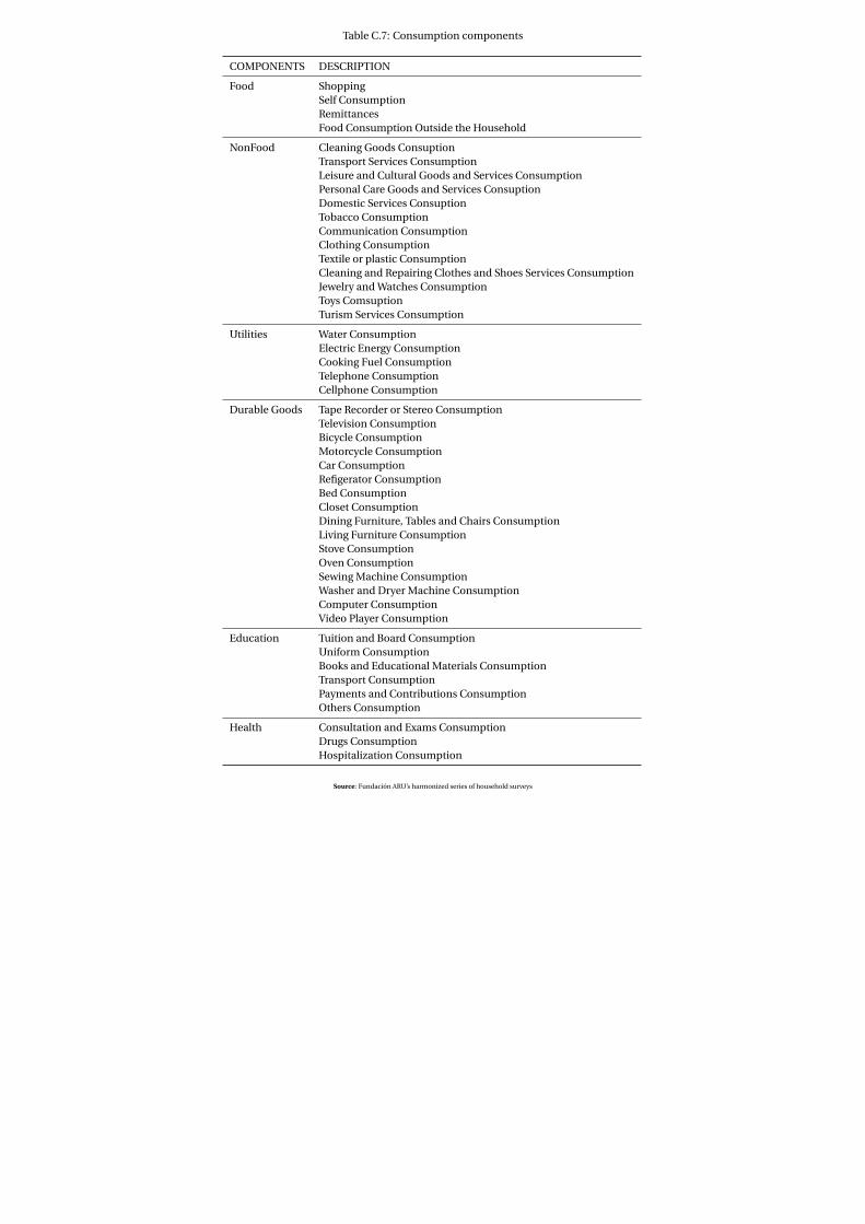
Table C.7: Consumption components

COMPONENTS DESCRIPTION

Food ShoppingSelf ConsumptionRemittancesFood Consumption Outside the Household

NonFood Cleaning Goods ConsuptionTransport Services ConsumptionLeisure and Cultural Goods and Services ConsumptionPersonal Care Goods and Services ConsuptionDomestic Services ConsuptionTobacco ConsumptionCommunication ConsumptionClothing ConsumptionTextile or plastic ConsumptionCleaning and Repairing Clothes and Shoes Services ConsumptionJewelry and Watches ConsumptionToys ComsuptionTurism Services Consumption

Utilities Water ConsumptionElectric Energy ConsumptionCooking Fuel ConsumptionTelephone ConsumptionCellphone Consumption

Durable Goods Tape Recorder or Stereo ConsumptionTelevision ConsumptionBicycle ConsumptionMotorcycle ConsumptionCar ConsumptionRefigerator ConsumptionBed ConsumptionCloset ConsumptionDining Furniture, Tables and Chairs ConsumptionLiving Furniture ConsumptionStove ConsumptionOven ConsumptionSewing Machine ConsumptionWasher and Dryer Machine ConsumptionComputer ConsumptionVideo Player Consumption

Education Tuition and Board ConsumptionUniform ConsumptionBooks and Educational Materials ConsumptionTransport ConsumptionPayments and Contributions ConsumptionOthers Consumption

Health Consultation and Exams ConsumptionDrugs ConsumptionHospitalization Consumption

Source: Fundación ARU’s harmonized series of household surveys

37

Table C.8: Income components

SOURCE DESCRIPTION

Labor Net Wage Income of Primary ActivityWage Income in Benefits of Primary ActivityTotal Wage Income in Kind of Primary ActivityNet Wage Income of Secondary ActivityTotal Wage Income in Benefits of Secondary ActivityTotal Wage Income in Kind of Secondary Activity

Interhousehold transfers Family assistanceInterior TransfersExterior Transfers

Properties InterestsImmovable Properties and Houses RentalAgricultural Properties RentalDividens, Utilities or Corporate RetreatsMachine and equipment rental

Social Security RetirementWar veteransDisabilityWidowhoodOther Rents

Other Compensation for leaving a jobInsurance CompensationOther Extraordinary Income

Source: Fundación ARU’s harmonized series of household surveys

38

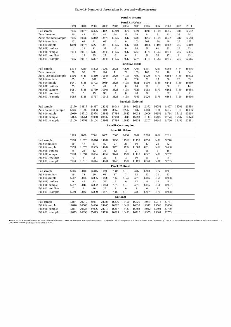
Table C.9: Number of observations by year and welfare measure

Panel A: Income

Panel A1: Urban1999 2000 2001 2002 2003 2004 2005 2006 2007 2008 2009 2011

Full sample 7036 10678 12425 14023 14209 15674 9324 11241 11322 8655 9345 22582Zero Incomes 20 43 83 48 34 27 38 34 2 23 33 34Zeros excluded sample 7016 10635 12342 13975 14175 15647 9286 11207 11320 8632 9312 22548P(0.01) outliers 17 63 71 62 0 0 103 201 128 50 29 129P(0.01) sample 6999 10572 12271 13913 14175 15647 9183 11006 11192 8582 9283 22419P(0.001) outliers 2 19 41 32 0 0 18 76 61 21 25 63P(0.001) sample 7014 10616 12301 13943 14175 15647 9268 11131 11259 8611 9287 22485P(0.0001) outliers 1 19 35 27 0 0 11 26 53 17 9 33P(0.0001) sample 7015 10616 12307 13948 14175 15647 9275 11181 11267 8615 9303 22515

Panel A2: Rural

Full sample 5134 8239 11892 10209 3834 4220 7208 5131 5230 6202 6164 10936Zero Incomes 28 96 82 164 11 22 109 102 51 10 14 34Zeros excluded sample 5106 8143 11810 10045 3823 4198 7099 5029 5179 6192 6150 10902P(0.01) outliers 65 5 107 76 0 0 268 29 13 50 20 33P(0.01) sample 5041 8138 11703 9969 3823 4198 6831 5000 5166 6142 6130 10869P(0.001) outliers 25 5 51 41 0 0 74 16 9 30 0 14P(0.001) sample 5081 8138 11759 10004 3823 4198 7025 5013 5170 6162 6150 10888P(0.0001) outliers 21 5 13 32 0 0 40 3 3 27 0 6P(0.0001) sample 5085 8138 11797 10013 3823 4198 7059 5026 5176 6165 6150 10896

Panel A3: National

Full sample 12170 18917 24317 24232 18043 19894 16532 16372 16552 14857 15509 33518Zero excluded sample 5126 8186 11893 10093 3857 4225 7137 5063 5181 6215 6183 10936P(0.01) sample 12040 18710 23974 23882 17998 19845 16014 16006 16358 14724 15413 33288P(0.001) sample 12095 18754 24060 23947 17998 19845 16293 16144 16429 14773 15437 33373P(0.0001) sample 12100 18754 24104 23961 17998 19845 16334 16207 16443 14780 15453 33411

Panel B: Consumption

Panel B1: Urban

1999 2000 2001 2002 2005 2006 2007 2008 2009 2011

Full sample 7178 11620 12616 14187 9453 11319 11439 8758 9436 22770P(0.01) outliers 19 47 61 80 27 25 56 27 26 82P(0.01) sample 7159 11573 12555 14107 9426 11294 11383 8731 9410 22688P(0.001) outliers 8 29 12 35 12 17 21 11 6 18P(0.001) sample 7170 11591 12604 14152 9441 11302 11418 8747 9430 22752P(0.0001) outliers 4 4 2 26 8 17 10 10 5 5P(0.0001) sample 7174 11616 12614 14161 9445 11302 11429 8748 9431 22765

Panel B2: Rural

Full sample 5706 9090 12415 10599 7383 5131 5287 6213 6177 10991P(0.01) outliers 19 74 80 61 17 7 12 27 21 23P(0.01) sample 5687 9016 12335 10538 7366 5124 5275 6186 6156 10968P(0.001) outliers 9 46 23 38 7 0 12 18 16 4P(0.001) sample 5697 9044 12392 10561 7376 5131 5275 6195 6161 10987P(0.0001) outliers 7 8 16 26 3 0 4 6 7 3P(0.0001) sample 5699 9082 12399 10573 7380 5131 5283 6207 6170 10988

National

Full sample 12884 20710 25031 24786 16836 16450 16726 14971 15613 33761P(0.01) sample 12846 20589 24890 24645 16792 16418 16658 14917 15566 33656P(0.001) sample 12867 20635 24996 24713 16817 16433 16693 14942 15591 33739P(0.0001) sample 12873 20698 25013 24734 16825 16433 16712 14955 15601 33753

Source: Fundación ARU’s harmonized series of household surveys. Note: Outliers were nominated using tha BACON algorithm, which computes a Mahalanobis distance and then uses a ¬2 test to nominate observations as outliers. For this test we used Æ =0.01,0.001,0.0001 yielding the three samples above.

39

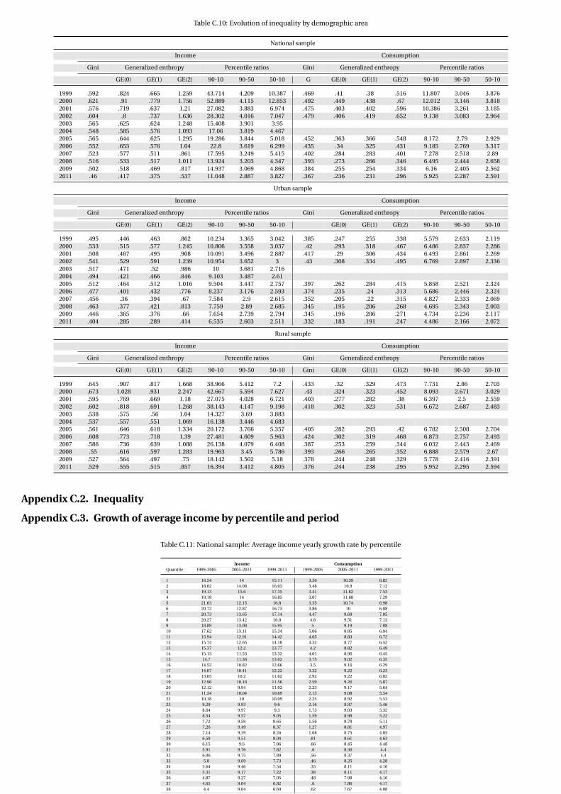
Table C.10: Evolution of inequality by demographic area

National sample

Income Consumption

Gini Generalized enthropy Percentile ratios Gini Generalized enthropy Percentile ratios

GE(0) GE(1) GE(2) 90-10 90-50 50-10 G GE(0) GE(1) GE(2) 90-10 90-50 50-10

1999 .592 .824 .665 1.259 43.714 4.209 10.387 .469 .41 .38 .516 11.807 3.046 3.8762000 .621 .91 .779 1.756 52.889 4.115 12.853 .492 .449 .438 .67 12.012 3.146 3.8182001 .576 .719 .637 1.21 27.082 3.883 6.974 .475 .403 .402 .596 10.386 3.261 3.1852002 .604 .8 .737 1.636 28.302 4.016 7.047 .479 .406 .419 .652 9.138 3.083 2.9642003 .565 .625 .624 1.248 15.408 3.901 3.952004 .548 .585 .576 1.093 17.06 3.819 4.4672005 .565 .644 .625 1.295 19.286 3.844 5.018 .452 .363 .366 .548 8.172 2.79 2.9292006 .552 .653 .576 1.04 22.8 3.619 6.299 .435 .34 .325 .431 9.185 2.769 3.3172007 .523 .577 .511 .861 17.595 3.249 5.415 .402 .284 .283 .401 7.278 2.518 2.892008 .516 .533 .517 1.011 13.924 3.203 4.347 .393 .273 .266 .346 6.495 2.444 2.6582009 .502 .518 .469 .817 14.937 3.069 4.868 .384 .255 .254 .334 6.16 2.405 2.5622011 .46 .417 .375 .537 11.048 2.887 3.827 .367 .236 .231 .296 5.925 2.287 2.591

Urban sample

Income Consumption


GE(0) GE(1) GE(2) 90-10 90-50 50-10 GE(0) GE(1) GE(2) 90-10 90-50 50-10

1999 .495 .446 .463 .862 10.234 3.365 3.042 .385 .247 .255 .338 5.579 2.633 2.1192000 .533 .515 .577 1.245 10.806 3.558 3.037 .42 .293 .318 .467 6.486 2.837 2.2862001 .508 .467 .495 .908 10.091 3.496 2.887 .417 .29 .306 .434 6.493 2.861 2.2692002 .541 .529 .591 1.239 10.954 3.652 3 .43 .308 .334 .495 6.769 2.897 2.3362003 .517 .471 .52 .986 10 3.681 2.7162004 .494 .421 .466 .846 9.103 3.487 2.612005 .512 .464 .512 1.016 9.504 3.447 2.757 .397 .262 .284 .415 5.858 2.521 2.3242006 .477 .401 .432 .776 8.237 3.176 2.593 .374 .235 .24 .313 5.686 2.446 2.3242007 .456 .36 .394 .67 7.584 2.9 2.615 .352 .205 .22 .315 4.827 2.333 2.0692008 .463 .377 .421 .813 7.759 2.89 2.685 .345 .195 .206 .268 4.695 2.343 2.0032009 .446 .365 .376 .66 7.654 2.739 2.794 .345 .196 .206 .271 4.734 2.236 2.1172011 .404 .285 .289 .414 6.535 2.603 2.511 .332 .183 .191 .247 4.486 2.166 2.072

Rural sample

Income Consumption


GE(0) GE(1) GE(2) 90-10 90-50 50-10 Gini GE(0) GE(1) GE(2) 90-10 90-50 50-10

1999 .645 .907 .817 1.668 38.966 5.412 7.2 .433 .32 .329 .473 7.731 2.86 2.7032000 .673 1.028 .931 2.247 42.667 5.594 7.627 .43 .324 .323 .452 8.093 2.671 3.0292001 .595 .769 .669 1.18 27.075 4.028 6.721 .403 .277 .282 .38 6.397 2.5 2.5592002 .602 .818 .691 1.268 38.143 4.147 9.198 .418 .302 .323 .531 6.672 2.687 2.4832003 .538 .575 .56 1.04 14.327 3.69 3.8832004 .537 .557 .551 1.069 16.138 3.446 4.6832005 .561 .646 .618 1.334 20.172 3.766 5.357 .405 .282 .293 .42 6.782 2.508 2.7042006 .608 .773 .718 1.39 27.481 4.609 5.963 .424 .302 .319 .468 6.873 2.757 2.4932007 .586 .736 .639 1.088 26.138 4.079 6.408 .387 .253 .259 .344 6.032 2.443 2.4692008 .55 .616 .597 1.283 19.963 3.45 5.786 .393 .266 .265 .352 6.888 2.579 2.672009 .527 .564 .497 .75 18.142 3.502 5.18 .378 .244 .248 .329 5.778 2.416 2.3912011 .529 .555 .515 .857 16.394 3.412 4.805 .376 .244 .238 .295 5.952 2.295 2.594

Appendix C.2. Inequality

Appendix C.3. Growth of average income by percentile and period

Table C.11: National sample: Average income yearly growth rate by percentile

Income ConsumptionQuantile 1999-2005 2005-2011 1999-2011 1999-2005 2005-2011 1999-2011

1 16.24 14 15.11 3.36 10.39 6.822 18.02 14.08 16.03 3.48 10.9 7.123 19.13 15.6 17.35 3.41 11.82 7.534 19.78 14 16.85 3.07 11.68 7.295 21.63 12.15 16.8 3.35 10.74 6.986 20.72 12.87 16.73 3.86 10 6.887 20.73 13.65 17.14 4.47 9.69 7.058 20.27 13.42 16.8 4.8 9.51 7.139 18.89 13.08 15.95 5 9.19 7.0810 17.62 13.11 15.34 5.06 8.85 6.9411 15.94 12.91 14.42 4.65 8.83 6.7212 15.74 12.65 14.18 4.32 8.77 6.5213 15.37 12.2 13.77 4.2 8.82 6.4914 15.13 11.53 13.32 4.01 8.96 6.4515 14.7 11.36 13.02 3.75 9.02 6.3516 14.52 10.82 12.66 3.5 9.16 6.2917 14.07 10.41 12.22 3.32 9.22 6.2318 13.05 10.2 11.62 2.92 9.22 6.0219 12.96 10.18 11.56 2.59 9.26 5.8720 12.12 9.94 11.02 2.23 9.17 5.6421 11.34 10.04 10.69 2.13 9.08 5.5422 10.18 10 10.09 2.25 8.92 5.5323 9.29 9.93 9.6 2.16 8.87 5.4624 8.64 9.97 9.3 1.73 9.03 5.3225 8.54 9.57 9.05 1.59 8.98 5.2226 7.72 9.59 8.65 1.56 8.78 5.1127 7.26 9.49 8.37 1.27 8.81 4.9728 7.14 9.39 8.26 1.08 8.75 4.8529 6.58 9.51 8.04 .81 8.61 4.6330 6.15 9.6 7.86 .66 8.45 4.4831 5.91 9.76 7.82 .6 8.36 4.432 6.06 9.75 7.89 .56 8.37 4.433 5.8 9.69 7.73 .46 8.25 4.2834 5.64 9.46 7.54 .35 8.11 4.1635 5.31 9.17 7.22 .38 8.11 4.1736 4.87 9.27 7.05 .48 7.98 4.1637 4.65 9.04 6.82 .6 7.86 4.1738 4.4 9.04 6.69 .62 7.67 4.0839 4.34 9.06 6.68 .52 7.56 3.9840 3.92 9.05 6.45 .51 7.43 3.9141 3.84 8.99 6.38 .36 7.36 3.842 3.81 8.87 6.31 .44 7.29 3.8143 3.68 8.76 6.19 .49 7.17 3.7744 3.64 8.58 6.08 .35 7.16 3.745 3.34 8.65 5.96 .31 7.13 3.6646 3.33 8.69 5.98 .13 7.06 3.5447 3.15 8.6 5.84 -.01 7.02 3.4448 3 8.49 5.71 -.09 7 3.3949 3 8.18 5.56 -.15 7 3.3750 3 8.14 5.54 -.09 6.83 3.3151 2.94 7.91 5.39 .02 6.69 3.352 2.79 7.81 5.27 .01 6.65 3.2853 2.89 7.61 5.22 -.13 6.64 3.254 2.82 7.53 5.15 -.25 6.54 3.0955 2.73 7.38 5.03 -.42 6.48 2.9856 2.59 7.24 4.89 -.44 6.43 2.9457 2.47 7.18 4.8 -.49 6.36 2.8858 2.56 7.09 4.8 -.51 6.24 2.8159 2.32 7.09 4.68 -.48 6.22 2.8260 2.22 7.08 4.62 -.56 6.16 2.7461 2.29 6.98 4.61 -.64 6.11 2.6862 2.17 6.94 4.53 -.72 6 2.5963 2.02 6.72 4.35 -.7 5.8 2.564 2.15 6.65 4.38 -.64 5.6 2.4365 2.02 6.57 4.27 -.52 5.39 2.3966 1.91 6.64 4.25 -.42 5.31 2.467 2 6.53 4.24 -.46 5.14 2.368 1.92 6.33 4.1 -.38 4.89 2.2269 1.79 6.39 4.07 -.29 4.79 2.2270 1.65 6.28 3.94 -.28 4.73 2.1971 1.55 6.18 3.84 -.39 4.73 2.1472 1.64 5.97 3.78 -.46 4.67 2.0773 1.64 5.92 3.76 -.71 4.73 1.9874 1.85 5.91 3.86 -.86 4.66 1.8675 1.96 5.74 3.83 -.96 4.51 1.7476 2.08 5.44 3.74 -.94 4.39 1.6977 1.9 5.31 3.59 -.92 4.31 1.6678 1.7 5.16 3.42 -.87 4.2 1.6479 1.33 5.14 3.22 -.78 4.16 1.6680 1.57 5 3.27 -.68 4.08 1.6781 1.42 4.9 3.15 -.61 3.88 1.6182 1.61 4.63 3.11 -.55 3.67 1.5483 1.72 4.26 2.98 -.85 3.7 1.484 1.5 4.05 2.77 -.85 3.64 1.3785 1.49 4.02 2.75 -1.06 3.61 1.2486 1.44 3.77 2.6 -1.2 3.47 1.1187 1.69 3.39 2.54 -1.49 3.37 .9188 1.47 3.39 2.42 -1.33 3.19 .989 1.9 3.17 2.53 -1.35 3.1 .8590 1.66 2.98 2.32 -1.43 3.19 .8691 1.49 2.87 2.18 -1.47 2.97 .7392 1.43 2.55 1.99 -1.25 2.6 .6693 1.72 1.89 1.81 -1.07 2.38 .6494 1.6 1.44 1.52 -1.14 2.01 .4295 1.78 .92 1.35 -.55 1.37 .496 2.2 .53 1.36 -.88 .95 .0397 2.92 .02 1.46 -.77 .49 -.1498 3.27 -.97 1.13 .31 -.52 -.1199 1.81 -1 .39 .75 -.3 .22100 4.22 -5.18 -.59 1.72 -1.64 .03

40

Table C.12: Urban sample: Average income yearly growth rate by percentile


1 10.94 11.25 11.1 4.12 3.88 42 5.68 11.13 8.37 -.18 4.64 2.23 4.44 8.04 6.23 -1.05 5.07 1.964 2.63 7.73 5.15 -1.06 5.87 2.355 2.29 7.26 4.75 -1.41 6.08 2.276 2.05 6.68 4.34 -1.57 5.89 2.097 2.3 7.02 4.63 -1.62 5.59 1.928 2.15 7.49 4.79 -2.1 6.07 1.919 1.75 8.14 4.9 -2.03 6.14 1.9710 2.16 7.81 4.95 -2.21 6.12 1.8711 2.17 7.73 4.91 -2.44 6.21 1.812 2.12 7.85 4.94 -2.1 5.99 1.8713 1.77 8.1 4.89 -1.77 5.84 1.9614 1.29 8.31 4.74 -1.66 5.86 2.0315 1.02 8.43 4.66 -1.49 5.77 2.0816 .93 8.65 4.72 -1.41 5.73 2.117 1.31 8.51 4.85 -1.42 5.75 2.118 1.44 8.29 4.81 -1.27 5.54 2.0819 1.36 8.06 4.66 -1.17 5.44 2.0820 1 8.17 4.52 -.96 5.38 2.1621 1.02 7.97 4.44 -.92 5.4 2.1922 1.03 7.96 4.44 -.91 5.45 2.2223 .74 8.17 4.39 -.9 5.44 2.2224 .58 8.29 4.36 -.96 5.28 2.1125 .86 8.07 4.41 -1.04 5.23 2.0426 .87 7.9 4.33 -1.13 5.25 2.0127 .83 7.86 4.28 -1.15 5.35 2.0528 .76 7.82 4.23 -1.24 5.38 2.0129 .66 7.82 4.18 -1.27 5.25 1.9430 .38 7.86 4.05 -1.19 5.25 1.9831 .32 7.71 3.95 -1.23 5.29 1.9832 .04 7.8 3.84 -1.26 5.24 1.9433 .28 7.69 3.92 -1.18 5.16 1.9434 .41 7.41 3.85 -1.3 5.03 1.8135 .41 7.18 3.74 -1.34 4.99 1.7736 .32 7.03 3.62 -1.4 5.1 1.837 .28 6.91 3.54 -1.48 5.11 1.7638 .29 6.87 3.52 -1.5 5.07 1.7339 .58 6.67 3.58 -1.46 5.11 1.7740 .49 6.67 3.53 -1.39 5.02 1.7741 .56 6.47 3.47 -1.42 5.01 1.7542 .52 6.31 3.37 -1.42 4.92 1.743 .53 6.29 3.37 -1.52 4.9 1.6444 .6 6.21 3.37 -1.53 4.83 1.645 .5 6.21 3.32 -1.6 4.8 1.5546 .27 6.21 3.2 -1.59 4.81 1.5647 .42 6.05 3.19 -1.49 4.62 1.5248 .54 5.96 3.21 -1.27 4.44 1.5449 .48 5.9 3.16 -1.12 4.33 1.5750 .56 5.85 3.18 -1.03 4.29 1.5951 .81 5.67 3.21 -1.09 4.19 1.5252 .82 5.71 3.24 -1.04 4.1 1.553 .68 5.65 3.14 -.99 4.04 1.554 .54 5.73 3.1 -.85 3.91 1.555 .64 5.62 3.1 -.9 3.75 1.456 .56 5.55 3.02 -.91 3.68 1.3657 .57 5.48 2.99 -.94 3.69 1.3458 .5 5.51 2.98 -1.08 3.69 1.2859 .45 5.37 2.88 -1.29 3.64 1.1560 .45 5.35 2.87 -1.34 3.6 1.161 .84 5.18 2.99 -1.48 3.68 1.0762 1.12 4.93 3 -1.63 3.67 .9963 1.14 4.89 3 -1.72 3.65 .9364 1.07 4.86 2.95 -1.71 3.59 .965 1.1 4.81 2.94 -1.54 3.52 .9666 1.19 4.48 2.82 -1.59 3.43 .8967 1.1 4.41 2.74 -1.44 3.3 .968 .64 4.38 2.49 -1.28 3.19 .9369 .69 4.2 2.43 -1.24 3.21 .9670 .85 4.14 2.48 -1.22 3.13 .9371 .8 4.12 2.44 -1.19 3.08 .9272 .7 3.96 2.32 -1.21 3.04 .8973 .95 3.73 2.33 -1.25 2.91 .8174 1.01 3.49 2.24 -1.29 2.9 .7975 1 3.31 2.15 -1.45 2.94 .7276 1.13 3.05 2.08 -1.46 2.8 .6577 1.18 2.97 2.07 -1.53 2.71 .5778 1.16 2.91 2.03 -1.63 2.75 .5479 1.21 2.73 1.97 -1.99 2.8 .3880 1.23 2.72 1.98 -1.93 2.77 .3981 1.43 2.44 1.94 -2.01 2.7 .3282 1.24 2.33 1.78 -1.95 2.5 .2583 1.38 2.18 1.78 -1.8 2.38 .2784 1.66 1.99 1.82 -1.83 2.36 .2585 1.39 1.84 1.61 -1.99 2.44 .286 1.16 2.02 1.59 -2.12 2.47 .1587 1.28 1.84 1.56 -1.9 2.14 .188 .96 1.8 1.38 -1.71 1.79 .0289 1.34 1.26 1.3 -1.48 1.73 .1190 1.24 1.04 1.14 -1.69 1.54 -.0991 1.17 .66 .92 -1.41 1.34 -.0592 1.4 .18 .79 -.96 .93 -.0293 1.41 -.05 .68 -1.01 .51 -.2694 1.89 -.28 .8 -1.43 .4 -.5295 2.28 -.77 .74 -1.23 .18 -.5396 3.08 -1.5 .76 -.65 -.56 -.697 2.72 -2.18 .24 .42 -1.27 -.4398 1.31 -1.65 -.18 .75 -.91 -.0899 1.71 -2.44 -.38 .55 -.64 -.05100 4.31 -6.71 -1.36 1.83 -2.33 -.27

41

Table C.13: Rural sample: Average income yearly growth rate by percentile


1 13.09 19.69 16.34 3.2 10.3 6.692 15.98 13.84 14.91 2.98 9.77 6.333 15.3 12.73 14.01 3.08 9.9 6.434 18.18 12.3 15.2 3.01 10.49 6.685 16.59 14.31 15.45 3.02 10.93 6.96 18.2 14.67 16.42 3.03 10.96 6.927 18.64 15.32 16.96 3.15 11.74 7.368 18.53 14.9 16.7 2.61 12.16 7.289 18.44 13.92 16.16 2.26 12.09 7.0710 19.45 12.84 16.1 2.47 11.94 7.111 20.68 12.73 16.64 2.54 11.67 7.0112 21.74 11.75 16.64 2.29 11.35 6.7313 21.55 11.07 16.19 2.51 10.88 6.6114 21.06 11.19 16.02 3.08 10.42 6.6915 20.65 11.88 16.19 3.2 10.33 6.7116 20.79 12.52 16.58 3.59 10.27 6.8817 20.9 13.03 16.9 3.7 10.25 6.9218 20.51 13.26 16.83 3.76 9.94 6.8119 20.72 13.33 16.96 3.88 10.02 6.9120 20.57 13.11 16.78 4.03 10.19 7.0621 20.31 12.6 16.39 4.36 9.85 7.0722 19.76 12.37 16.01 4.43 9.7 7.0323 19.34 12.35 15.79 4.53 9.54 7.0124 18.16 12.83 15.47 4.63 9.47 7.0225 18.68 12.63 15.62 4.42 9.47 6.9126 17.7 12.59 15.12 4.38 9.4 6.8627 16.32 12.84 14.57 4.35 9.41 6.8528 16.54 12.9 14.71 4.24 9.32 6.7529 16.46 12.82 14.63 4.09 9.3 6.6630 16.22 12.91 14.56 4.09 9.49 6.7531 15.94 12.97 14.45 4.17 9.63 6.8732 15.73 12.86 14.29 4.13 9.76 6.9133 15.7 12.51 14.1 4.15 9.69 6.8934 15.47 12.27 13.86 4.11 9.71 6.8835 15.69 12.24 13.95 4.02 9.94 6.9436 15.87 12.05 13.94 3.82 10.24 6.9837 15.74 11.95 13.83 3.77 10.33 738 15.87 11.73 13.78 3.74 10.43 7.0339 15.65 11.32 13.46 3.81 10.37 7.0440 16.03 11.17 13.57 3.98 10.28 7.0841 16.08 11.26 13.64 3.65 10.34 6.9442 15.63 11.14 13.37 3.47 10.35 6.8543 14.88 11.08 12.96 3.27 10.47 6.8144 14.12 11.24 12.67 3.27 10.51 6.8345 14.44 11.22 12.82 3.09 10.56 6.7646 14.73 11.44 13.07 2.92 10.61 6.6947 14.58 11.39 12.98 2.79 10.73 6.6848 14.11 11.32 12.71 2.67 10.83 6.6749 14.01 11.47 12.73 2.68 10.85 6.6950 13.82 11.29 12.55 2.66 11 6.7551 14.1 10.84 12.46 2.65 11 6.7452 14.06 10.57 12.3 2.51 11.11 6.7253 14.02 10.19 12.09 2.44 11.1 6.6854 13.68 10.15 11.9 2.46 10.89 6.5955 13.41 10.15 11.77 2.46 10.88 6.5956 13.1 10.12 11.6 2.45 10.99 6.6357 12.5 10.11 11.3 2.56 10.97 6.6858 12.23 10.36 11.29 2.57 10.87 6.6459 11.77 10.63 11.2 2.55 10.8 6.660 11.95 10.65 11.29 2.52 11.08 6.7161 11.66 10.57 11.12 2.39 11.12 6.6762 11.28 10.71 10.99 2.25 11.12 6.5963 11.21 10.43 10.82 2.23 10.95 6.564 11.75 10.09 10.92 2.13 10.88 6.4165 11.54 10.09 10.81 2.03 10.87 6.3666 10.78 10.11 10.44 2.15 10.77 6.3867 10.43 10.14 10.29 2.11 10.73 6.3368 10.45 9.99 10.22 2.19 10.75 6.3969 10.6 10.06 10.33 2.12 10.67 6.3170 10.85 10.12 10.48 2.14 10.52 6.2571 10.75 10.22 10.48 2.13 10.44 6.272 10.45 9.89 10.17 2.26 10.29 6.273 9.67 9.7 9.68 2.34 10.2 6.274 9.72 9.77 9.75 2.13 10.39 6.1875 9.43 9.86 9.65 1.85 10.31 676 9.08 9.9 9.49 1.64 10.17 5.8277 8.8 9.88 9.34 1.51 10.06 5.778 8.66 9.91 9.28 1.61 9.85 5.6579 9.21 9.6 9.4 1.47 9.84 5.5780 9.63 9.46 9.54 1.25 9.88 5.4881 10.13 9.64 9.88 1.5 9.77 5.5682 9.75 9.48 9.61 1.55 9.52 5.4683 9.06 9.5 9.28 1.56 9.48 5.4484 8.65 9.51 9.08 1.48 9.42 5.3785 8.73 9.35 9.04 1.39 9.48 5.3686 8.9 9.42 9.16 1.21 9.39 5.2287 9.2 9.08 9.14 1.06 9.36 5.1388 9.09 9.04 9.07 .88 9.58 5.1489 8.91 8.96 8.94 .87 9.49 5.0990 8 9.19 8.59 .45 9.45 4.8591 7.25 9.48 8.36 .42 9.36 4.7992 6.56 9.98 8.26 .37 8.95 4.5793 6.09 10.16 8.11 .11 8.6 4.2794 5.4 10.12 7.73 .73 8.19 4.495 5.45 9.75 7.58 .95 8.29 4.5696 4.8 10.78 7.75 .7 8.26 4.4197 3.91 10.75 7.28 1.16 8.4 4.7298 2.23 10.89 6.47 1.7 7.8 4.7199 3.18 9.55 6.32 1.54 7.09 4.28100 7.16 3.78 5.46 1.69 4.42 3.05

42

Figure C.15: Evolution of income and consumption inequality measured by generalized entropy measures

0

.5

1

1.5

2

2.5

GE

inde

xes

1999 2001 2003 2005 2007 2009 2011

GE(0) GE(1) GE(2)

National

0

.5

1

1.5

2

2.5

GE

inde

xes

1999 2001 2003 2005 2007 2009 2011

GE(0) GE(1) GE(2)

Urban

0

.5

1

1.5

2

2.5

GE

inde

xes

1999 2001 2003 2005 2007 2009 2011

GE(0) GE(1) GE(2)

Rural

Income

.2

.3

.4

.5

.6

.7

GE

inde

xes

1999 2001 2003 2005 2007 2009 2011

GE(0) GE(1) GE(2)

National

.2

.3

.4

.5

.6

.7G

E in

dexe

s

1999 2001 2003 2005 2007 2009 2011

GE(0) GE(1) GE(2)

Urban

.2

.3

.4

.5

.6

.7

GE

inde

xes

1999 2001 2003 2005 2007 2009 2011

GE(0) GE(1) GE(2)

Rural

Consumption

43

Appendix C.4. Lorenz curves

Table C.14: National sample: Income Lorenz curves by year

Quantile 1999 2000 2001 2002 2003 2004 2005 2006 2007 2008 2009 2011

1 0 0 0 0 0 0 0 0 0 0 0 02 0 0 0 0 0 .001 0 0 0 0 0 .0013 0 0 0 0 .001 .001 .001 0 .001 .001 .001 .0014 0 0 .001 .001 .001 .002 .001 .001 .001 .001 .001 .0025 .001 .001 .001 .001 .002 .002 .002 .001 .002 .002 .002 .0036 .001 .001 .002 .001 .003 .003 .002 .002 .002 .003 .003 .0047 .001 .001 .002 .002 .004 .004 .003 .002 .003 .004 .004 .0068 .002 .001 .003 .002 .005 .005 .004 .003 .004 .005 .005 .0079 .002 .002 .003 .003 .006 .006 .005 .004 .005 .006 .006 .00910 .002 .002 .004 .003 .008 .007 .006 .005 .006 .008 .007 .0111 .003 .003 .005 .004 .009 .009 .007 .006 .007 .009 .009 .01212 .004 .003 .006 .005 .011 .01 .009 .007 .009 .011 .01 .01413 .004 .004 .007 .006 .012 .012 .01 .008 .01 .013 .012 .01714 .005 .004 .008 .007 .014 .014 .011 .01 .012 .015 .014 .01915 .006 .005 .009 .008 .016 .015 .013 .011 .014 .017 .016 .02216 .007 .006 .011 .01 .018 .017 .015 .013 .016 .019 .018 .02417 .008 .006 .012 .011 .02 .02 .017 .014 .018 .021 .02 .02718 .009 .007 .014 .012 .022 .022 .019 .016 .02 .024 .023 .0319 .01 .008 .016 .014 .024 .024 .021 .018 .023 .026 .025 .03320 .012 .01 .017 .016 .027 .027 .023 .02 .025 .029 .028 .03621 .013 .011 .019 .018 .029 .029 .025 .023 .028 .032 .031 .0422 .015 .012 .022 .02 .031 .032 .028 .025 .03 .034 .034 .04323 .016 .014 .024 .022 .034 .035 .03 .027 .033 .037 .037 .04724 .018 .015 .026 .024 .037 .037 .033 .03 .036 .041 .04 .0525 .02 .017 .029 .026 .039 .04 .036 .033 .039 .044 .043 .05426 .022 .019 .031 .028 .042 .043 .039 .036 .043 .047 .047 .05827 .025 .021 .034 .031 .045 .047 .042 .039 .046 .051 .05 .06228 .027 .024 .037 .033 .048 .05 .045 .042 .049 .054 .054 .06729 .03 .026 .039 .036 .051 .053 .048 .045 .053 .058 .058 .07130 .032 .028 .043 .039 .054 .057 .051 .048 .057 .062 .062 .07631 .035 .031 .046 .041 .058 .06 .054 .052 .06 .066 .066 .0832 .038 .034 .049 .044 .061 .064 .058 .055 .064 .07 .07 .08533 .041 .036 .052 .048 .065 .068 .061 .059 .068 .074 .075 .0934 .044 .039 .056 .051 .068 .071 .065 .063 .073 .078 .079 .09535 .047 .042 .06 .054 .072 .075 .069 .066 .077 .083 .084 .136 .05 .045 .063 .058 .076 .079 .073 .07 .081 .087 .088 .10637 .054 .049 .067 .061 .08 .084 .077 .075 .086 .092 .093 .11138 .058 .052 .071 .065 .084 .088 .081 .079 .09 .097 .098 .11739 .062 .055 .075 .069 .088 .093 .085 .083 .095 .102 .103 .12240 .066 .059 .08 .073 .092 .097 .089 .088 .1 .107 .109 .12841 .07 .063 .084 .077 .096 .102 .093 .092 .105 .112 .114 .13442 .074 .067 .089 .081 .101 .107 .098 .097 .11 .117 .119 .1443 .078 .071 .093 .085 .105 .111 .102 .102 .116 .123 .125 .14644 .083 .076 .098 .09 .11 .116 .107 .107 .121 .128 .131 .15245 .087 .08 .103 .094 .115 .122 .112 .112 .127 .134 .137 .15946 .092 .085 .108 .099 .12 .127 .117 .117 .133 .14 .143 .16547 .097 .09 .113 .104 .125 .132 .122 .123 .139 .146 .149 .17248 .102 .095 .118 .109 .13 .138 .127 .129 .145 .152 .155 .17949 .108 .1 .124 .114 .136 .143 .133 .134 .151 .158 .162 .18650 .113 .105 .129 .119 .141 .149 .138 .14 .158 .164 .168 .19351 .119 .11 .135 .124 .147 .155 .144 .146 .164 .171 .175 .252 .124 .116 .141 .13 .153 .161 .15 .153 .171 .177 .182 .20853 .13 .121 .147 .135 .158 .167 .156 .159 .178 .184 .189 .21554 .136 .127 .153 .141 .165 .173 .162 .165 .185 .191 .196 .22355 .143 .133 .159 .147 .171 .179 .168 .172 .192 .198 .204 .23156 .149 .14 .166 .153 .177 .186 .175 .179 .2 .206 .212 .23957 .156 .146 .173 .159 .183 .193 .181 .186 .208 .213 .219 .24758 .163 .153 .18 .166 .19 .2 .188 .193 .215 .221 .228 .25659 .17 .159 .187 .172 .197 .207 .195 .201 .223 .228 .236 .26460 .178 .166 .194 .179 .204 .214 .203 .209 .231 .236 .245 .27361 .185 .173 .201 .186 .211 .221 .21 .217 .24 .245 .253 .28262 .193 .18 .209 .193 .218 .229 .218 .225 .248 .253 .262 .29163 .202 .188 .217 .201 .226 .237 .225 .233 .257 .262 .271 .30164 .21 .195 .225 .208 .233 .245 .234 .242 .266 .271 .281 .3165 .219 .203 .233 .216 .241 .253 .242 .25 .275 .28 .29 .3266 .227 .211 .242 .224 .249 .262 .25 .259 .284 .289 .3 .3367 .237 .22 .25 .232 .258 .271 .259 .269 .294 .298 .31 .3468 .246 .228 .259 .241 .267 .28 .268 .278 .303 .308 .32 .35169 .256 .237 .269 .249 .275 .289 .277 .288 .313 .318 .331 .36270 .266 .246 .278 .258 .285 .298 .286 .298 .323 .328 .341 .37271 .276 .255 .288 .267 .294 .308 .296 .308 .334 .339 .352 .38472 .286 .265 .298 .277 .304 .318 .306 .319 .344 .35 .363 .39573 .297 .275 .309 .287 .314 .328 .316 .33 .355 .361 .375 .40774 .309 .285 .319 .297 .324 .339 .327 .341 .367 .372 .387 .41975 .32 .296 .331 .307 .334 .35 .337 .353 .378 .383 .399 .43176 .332 .307 .342 .318 .345 .361 .349 .364 .39 .395 .411 .44477 .344 .319 .354 .329 .357 .373 .361 .377 .402 .408 .424 .45778 .357 .33 .366 .341 .368 .385 .373 .39 .415 .42 .437 .4779 .37 .343 .379 .353 .381 .397 .385 .403 .428 .433 .45 .48380 .384 .355 .392 .365 .393 .41 .398 .416 .441 .447 .464 .49781 .399 .368 .406 .378 .406 .424 .412 .43 .455 .461 .478 .51282 .414 .382 .421 .391 .42 .438 .426 .445 .47 .475 .492 .52783 .43 .396 .436 .405 .434 .453 .44 .46 .485 .49 .507 .54284 .446 .411 .451 .42 .449 .468 .456 .476 .501 .505 .523 .55885 .464 .427 .468 .435 .464 .484 .472 .492 .517 .521 .539 .57586 .482 .444 .485 .451 .481 .501 .489 .509 .535 .538 .556 .59287 .501 .461 .503 .468 .498 .519 .507 .527 .552 .555 .574 .6188 .521 .48 .522 .486 .515 .537 .525 .546 .571 .573 .593 .62889 .542 .5 .542 .505 .535 .557 .545 .566 .591 .592 .612 .64790 .564 .52 .563 .525 .555 .578 .566 .587 .612 .612 .632 .66891 .588 .543 .586 .547 .578 .601 .589 .61 .634 .633 .654 .68992 .614 .568 .61 .57 .602 .625 .612 .634 .657 .656 .676 .71193 .642 .594 .637 .596 .628 .651 .638 .66 .682 .68 .7 .73594 .672 .624 .666 .625 .658 .68 .667 .689 .709 .706 .726 .7695 .705 .657 .699 .658 .69 .711 .698 .72 .739 .733 .754 .78796 .741 .695 .736 .695 .726 .746 .733 .755 .772 .764 .785 .81697 .781 .738 .776 .739 .769 .786 .773 .794 .809 .799 .819 .84898 .828 .787 .825 .792 .82 .833 .822 .84 .851 .839 .859 .88599 .889 .855 .885 .862 .886 .893 .88 .899 .904 .89 .909 .93100 1 1 1 1 1 1 1 1 1 1 1 1

44

Table C.15: National sample: Consumption Lorenz curves by year

Quantile 1999 2000 2001 2002 2005 2006 2007 2008 2009 2011

1 .001 .001 .001 .001 .001 .001 .001 .001 .001 .0012 .001 .001 .002 .002 .002 .002 .002 .002 .002 .0033 .002 .002 .003 .003 .003 .003 .004 .004 .004 .0044 .003 .003 .004 .004 .004 .005 .006 .005 .006 .0065 .005 .004 .006 .006 .006 .006 .008 .007 .008 .0096 .006 .005 .007 .007 .008 .008 .01 .009 .011 .0117 .008 .007 .009 .009 .009 .01 .012 .012 .013 .0148 .009 .008 .011 .011 .011 .012 .014 .014 .016 .0169 .011 .01 .013 .013 .014 .014 .017 .017 .019 .01910 .012 .011 .015 .015 .016 .016 .019 .02 .022 .02211 .014 .013 .017 .018 .018 .019 .022 .023 .025 .02512 .016 .015 .019 .02 .021 .021 .025 .026 .029 .02913 .018 .017 .021 .022 .024 .024 .028 .029 .032 .03214 .021 .019 .024 .025 .027 .026 .031 .032 .036 .03615 .023 .022 .026 .028 .029 .029 .035 .036 .039 .0416 .025 .024 .029 .03 .032 .032 .038 .04 .043 .04417 .028 .027 .032 .033 .036 .035 .042 .043 .047 .04818 .03 .029 .035 .036 .039 .038 .045 .047 .051 .05219 .033 .032 .038 .039 .042 .041 .049 .051 .055 .05720 .036 .035 .041 .042 .045 .045 .053 .056 .059 .06121 .039 .038 .044 .046 .049 .048 .058 .06 .064 .06622 .042 .041 .047 .049 .053 .052 .062 .064 .068 .07123 .046 .044 .051 .052 .056 .056 .066 .069 .073 .07524 .049 .047 .054 .056 .06 .06 .07 .073 .077 .0825 .053 .051 .058 .06 .064 .064 .075 .078 .082 .08526 .056 .054 .062 .063 .068 .068 .08 .083 .087 .09127 .06 .058 .065 .067 .072 .072 .085 .088 .092 .09628 .064 .062 .069 .071 .076 .076 .09 .093 .097 .10129 .068 .066 .074 .075 .081 .081 .095 .098 .102 .10730 .072 .07 .078 .08 .085 .085 .1 .104 .108 .11331 .077 .074 .082 .084 .09 .09 .105 .109 .113 .11932 .081 .078 .087 .088 .094 .095 .111 .114 .119 .12433 .086 .083 .091 .093 .099 .1 .117 .12 .125 .1334 .09 .087 .096 .097 .104 .105 .122 .126 .131 .13735 .095 .092 .101 .102 .109 .11 .128 .132 .137 .14336 .1 .096 .106 .107 .114 .116 .134 .138 .143 .14937 .105 .101 .111 .112 .12 .121 .14 .144 .149 .15638 .111 .106 .116 .117 .125 .127 .146 .15 .155 .16339 .116 .111 .121 .122 .131 .132 .153 .156 .162 .16940 .121 .116 .126 .127 .136 .138 .159 .163 .168 .17641 .127 .122 .132 .133 .142 .144 .166 .169 .175 .18342 .133 .127 .137 .138 .148 .15 .172 .176 .182 .1943 .139 .133 .143 .144 .154 .156 .179 .183 .189 .19744 .145 .139 .149 .149 .16 .163 .186 .19 .196 .20545 .151 .145 .155 .155 .167 .169 .193 .197 .203 .21246 .157 .151 .16 .161 .173 .176 .2 .204 .21 .2247 .164 .157 .167 .167 .18 .183 .208 .212 .218 .22848 .17 .163 .173 .173 .186 .19 .215 .219 .225 .23549 .177 .169 .179 .18 .193 .197 .223 .227 .233 .24350 .184 .176 .186 .186 .2 .204 .23 .234 .241 .25151 .191 .183 .192 .193 .207 .212 .238 .242 .249 .2652 .198 .19 .199 .2 .214 .219 .246 .25 .257 .26853 .205 .197 .206 .207 .222 .227 .254 .258 .265 .27654 .213 .204 .214 .214 .229 .235 .262 .267 .274 .28555 .221 .211 .221 .221 .237 .243 .271 .275 .282 .29456 .229 .219 .228 .229 .245 .252 .279 .284 .291 .30357 .237 .226 .236 .236 .252 .26 .288 .293 .3 .31258 .245 .234 .244 .244 .261 .269 .297 .302 .308 .32159 .254 .242 .252 .252 .269 .278 .306 .311 .317 .3360 .262 .25 .26 .26 .277 .287 .315 .32 .327 .3461 .271 .259 .268 .269 .286 .296 .324 .329 .336 .34962 .28 .267 .277 .277 .295 .305 .334 .339 .346 .35963 .29 .276 .286 .286 .304 .315 .343 .349 .355 .36964 .299 .285 .295 .295 .313 .325 .353 .358 .365 .37965 .309 .294 .304 .304 .323 .335 .363 .369 .375 .3966 .319 .303 .313 .313 .333 .345 .373 .379 .386 .467 .329 .313 .323 .323 .343 .356 .384 .39 .396 .41168 .34 .323 .333 .332 .353 .366 .394 .4 .407 .42169 .35 .333 .343 .342 .364 .377 .405 .411 .418 .43270 .361 .343 .353 .352 .374 .388 .416 .423 .429 .44471 .373 .354 .364 .363 .385 .4 .427 .434 .44 .45572 .384 .365 .375 .373 .397 .411 .439 .446 .452 .46773 .396 .376 .386 .384 .408 .423 .451 .457 .464 .47974 .408 .388 .397 .395 .42 .436 .462 .469 .476 .49175 .421 .4 .409 .407 .432 .448 .474 .481 .488 .50376 .434 .412 .421 .419 .444 .461 .487 .494 .501 .51677 .447 .424 .434 .431 .457 .475 .499 .507 .513 .52878 .461 .437 .447 .443 .47 .488 .512 .52 .526 .54279 .475 .45 .46 .456 .484 .502 .525 .534 .54 .55580 .489 .464 .474 .47 .497 .516 .539 .548 .554 .56981 .504 .478 .488 .483 .512 .531 .553 .562 .567 .58382 .519 .493 .503 .497 .526 .546 .567 .577 .582 .59783 .534 .507 .518 .512 .541 .562 .582 .592 .597 .61284 .551 .523 .534 .527 .557 .578 .597 .607 .612 .62785 .568 .539 .551 .543 .573 .595 .613 .623 .628 .64386 .585 .556 .568 .559 .59 .612 .629 .639 .644 .65987 .604 .573 .587 .576 .607 .63 .646 .655 .661 .67588 .623 .592 .606 .594 .625 .648 .664 .672 .678 .69289 .644 .611 .626 .613 .644 .667 .682 .69 .696 .70990 .665 .632 .647 .633 .663 .688 .701 .709 .715 .72891 .686 .653 .669 .654 .683 .709 .721 .728 .734 .74792 .71 .676 .693 .677 .705 .731 .743 .749 .755 .76793 .734 .7 .717 .701 .728 .754 .765 .771 .776 .78894 .761 .726 .744 .728 .753 .778 .788 .794 .798 .8195 .789 .756 .773 .756 .78 .805 .813 .819 .822 .83396 .82 .789 .804 .789 .81 .833 .84 .846 .848 .85797 .854 .826 .839 .825 .843 .864 .869 .875 .876 .88498 .891 .868 .879 .868 .881 .899 .902 .907 .908 .91399 .934 .919 .927 .921 .926 .94 .941 .944 .945 .948100 1 1 1 1 1 1 1 1 1 1

45

Table C.17: Urban sample: Income Lorenz curves by year

Quantile 1999 2000 2001 2002 2003 2004 2005 2006 2007 2008 2009 2011

1 0 0 0 0 0 .001 0 0 .001 .001 0 .0012 .001 .001 .001 .001 .001 .002 .001 .002 .002 .002 .001 .0023 .002 .002 .002 .002 .003 .003 .002 .003 .004 .003 .002 .0044 .003 .003 .003 .003 .004 .005 .004 .004 .005 .005 .004 .0065 .005 .004 .004 .004 .005 .007 .005 .006 .007 .006 .006 .0086 .006 .005 .006 .006 .007 .008 .007 .008 .009 .008 .008 .017 .008 .007 .007 .007 .009 .01 .009 .01 .011 .01 .01 .0128 .01 .009 .009 .009 .011 .013 .011 .012 .014 .013 .012 .0159 .012 .01 .011 .011 .013 .015 .013 .015 .016 .015 .014 .01810 .014 .012 .013 .012 .015 .017 .015 .017 .019 .017 .017 .02111 .016 .014 .015 .014 .017 .019 .017 .02 .021 .02 .019 .02412 .018 .016 .018 .016 .019 .022 .019 .022 .024 .023 .022 .02713 .021 .018 .02 .018 .022 .024 .022 .025 .027 .025 .025 .0314 .023 .021 .022 .021 .024 .027 .024 .028 .03 .028 .028 .03415 .026 .023 .025 .023 .027 .03 .027 .031 .033 .031 .031 .03816 .028 .025 .028 .025 .029 .033 .029 .034 .036 .034 .034 .04117 .031 .028 .03 .028 .032 .036 .032 .037 .039 .038 .038 .04518 .034 .03 .033 .031 .035 .039 .035 .04 .043 .041 .041 .04919 .037 .033 .036 .033 .038 .042 .038 .043 .046 .044 .045 .05320 .04 .036 .039 .036 .041 .045 .041 .046 .049 .048 .048 .05721 .043 .039 .042 .039 .044 .048 .044 .05 .053 .051 .052 .06222 .046 .042 .045 .042 .047 .052 .047 .053 .057 .055 .056 .06623 .05 .045 .049 .045 .05 .055 .05 .057 .061 .059 .06 .07124 .053 .049 .052 .048 .053 .059 .053 .061 .064 .063 .064 .07525 .056 .052 .056 .051 .057 .062 .056 .064 .069 .066 .068 .0826 .06 .055 .059 .055 .06 .066 .06 .068 .073 .07 .072 .08527 .064 .059 .063 .058 .064 .07 .063 .072 .077 .075 .076 .08928 .067 .062 .066 .061 .067 .074 .067 .076 .081 .079 .081 .09429 .071 .066 .07 .065 .071 .078 .071 .08 .086 .083 .085 .130 .075 .07 .074 .069 .075 .082 .074 .084 .09 .088 .09 .10531 .079 .074 .078 .072 .079 .086 .078 .089 .095 .092 .095 .1132 .084 .078 .082 .076 .083 .09 .082 .093 .1 .097 .099 .11533 .088 .082 .087 .08 .087 .094 .086 .098 .105 .102 .104 .12134 .092 .086 .091 .084 .092 .099 .09 .102 .11 .107 .109 .12635 .097 .09 .095 .088 .096 .103 .094 .107 .115 .112 .115 .13236 .101 .094 .1 .092 .1 .108 .099 .112 .12 .117 .12 .13837 .106 .099 .104 .096 .105 .112 .103 .117 .126 .122 .125 .14438 .111 .103 .109 .101 .109 .117 .107 .122 .131 .127 .131 .1539 .116 .108 .114 .105 .114 .122 .112 .127 .137 .133 .136 .15640 .121 .112 .119 .109 .119 .127 .117 .132 .142 .138 .142 .16241 .126 .117 .124 .114 .124 .132 .122 .137 .148 .144 .148 .16842 .132 .122 .129 .119 .128 .137 .127 .143 .154 .149 .154 .17543 .137 .127 .134 .123 .134 .142 .132 .148 .16 .155 .16 .18144 .143 .132 .139 .128 .139 .148 .137 .154 .166 .161 .167 .18845 .148 .137 .145 .133 .144 .153 .142 .16 .172 .167 .173 .19546 .154 .142 .15 .139 .149 .159 .148 .166 .178 .173 .18 .20247 .16 .148 .156 .144 .155 .164 .153 .172 .185 .179 .187 .20948 .166 .153 .162 .149 .16 .17 .159 .178 .191 .186 .194 .21649 .172 .159 .168 .155 .166 .176 .165 .184 .198 .192 .201 .22350 .179 .164 .174 .16 .172 .182 .171 .191 .205 .199 .208 .2351 .185 .17 .18 .166 .178 .188 .177 .197 .211 .206 .215 .23852 .192 .176 .186 .171 .184 .195 .183 .204 .218 .213 .223 .24653 .198 .182 .193 .177 .19 .201 .189 .211 .225 .22 .23 .25354 .205 .188 .199 .183 .196 .208 .196 .218 .233 .227 .238 .26155 .212 .195 .206 .189 .202 .214 .202 .225 .24 .234 .245 .2756 .219 .201 .213 .196 .209 .221 .209 .232 .247 .242 .253 .27857 .227 .208 .22 .202 .216 .228 .216 .239 .255 .249 .261 .28658 .234 .214 .227 .209 .223 .235 .223 .247 .263 .257 .27 .29559 .242 .221 .234 .216 .23 .243 .23 .255 .271 .265 .278 .30360 .249 .228 .242 .222 .237 .25 .238 .262 .279 .273 .287 .31261 .257 .236 .249 .23 .244 .258 .245 .27 .287 .282 .295 .32162 .265 .243 .257 .237 .252 .265 .253 .279 .295 .29 .304 .33163 .273 .25 .265 .244 .259 .273 .261 .287 .304 .299 .313 .3464 .282 .258 .273 .252 .267 .282 .269 .296 .313 .308 .322 .3565 .29 .266 .282 .26 .275 .29 .277 .304 .321 .317 .332 .35966 .299 .274 .29 .268 .283 .299 .286 .313 .33 .326 .341 .36967 .308 .283 .299 .276 .292 .307 .295 .323 .34 .335 .351 .37968 .318 .291 .308 .284 .3 .316 .304 .332 .349 .345 .361 .3969 .327 .3 .317 .293 .309 .326 .313 .342 .359 .355 .371 .470 .337 .309 .327 .302 .318 .335 .322 .351 .369 .365 .381 .41171 .348 .318 .337 .311 .328 .345 .332 .362 .379 .375 .391 .42272 .358 .327 .347 .32 .337 .355 .342 .372 .389 .386 .402 .43373 .369 .337 .357 .33 .347 .365 .352 .383 .4 .397 .413 .44574 .38 .347 .368 .34 .357 .376 .363 .394 .411 .408 .424 .45675 .391 .358 .379 .35 .368 .387 .374 .405 .422 .42 .435 .46876 .404 .368 .39 .361 .379 .398 .386 .416 .434 .432 .447 .48177 .416 .38 .402 .371 .39 .41 .398 .428 .446 .444 .459 .49378 .428 .391 .414 .382 .402 .422 .41 .441 .458 .456 .472 .50679 .441 .403 .426 .394 .413 .434 .423 .453 .471 .469 .485 .51980 .454 .416 .439 .406 .426 .447 .436 .466 .484 .482 .498 .53381 .469 .429 .452 .418 .438 .46 .449 .48 .497 .495 .511 .54782 .483 .442 .466 .431 .452 .474 .464 .493 .511 .509 .526 .56183 .498 .455 .48 .445 .465 .489 .478 .508 .525 .523 .54 .57684 .513 .47 .496 .459 .48 .504 .493 .523 .54 .538 .555 .59185 .529 .485 .511 .473 .495 .52 .509 .539 .556 .554 .571 .60786 .546 .501 .528 .489 .511 .536 .526 .555 .572 .57 .587 .62487 .563 .517 .545 .505 .528 .554 .543 .572 .588 .587 .603 .64188 .582 .534 .563 .523 .547 .572 .561 .59 .606 .604 .621 .65989 .602 .553 .582 .541 .566 .591 .58 .609 .624 .622 .639 .67790 .622 .573 .603 .561 .586 .612 .6 .629 .643 .642 .658 .69691 .644 .595 .625 .582 .608 .634 .622 .65 .664 .661 .679 .71692 .668 .617 .649 .606 .632 .658 .645 .673 .685 .683 .7 .73793 .692 .643 .674 .631 .658 .683 .67 .697 .708 .705 .723 .75994 .718 .67 .701 .659 .686 .71 .696 .723 .734 .729 .746 .78295 .747 .7 .731 .69 .717 .739 .725 .751 .762 .755 .772 .80696 .777 .732 .764 .726 .752 .771 .758 .783 .792 .783 .801 .83397 .813 .767 .801 .767 .792 .808 .797 .818 .826 .815 .833 .86398 .855 .812 .845 .816 .84 .851 .839 .859 .864 .851 .87 .89799 .908 .876 .899 .881 .9 .905 .891 .91 .913 .899 .916 .936100 1 1 1 1 1 1 1 1 1 1 1 1

46

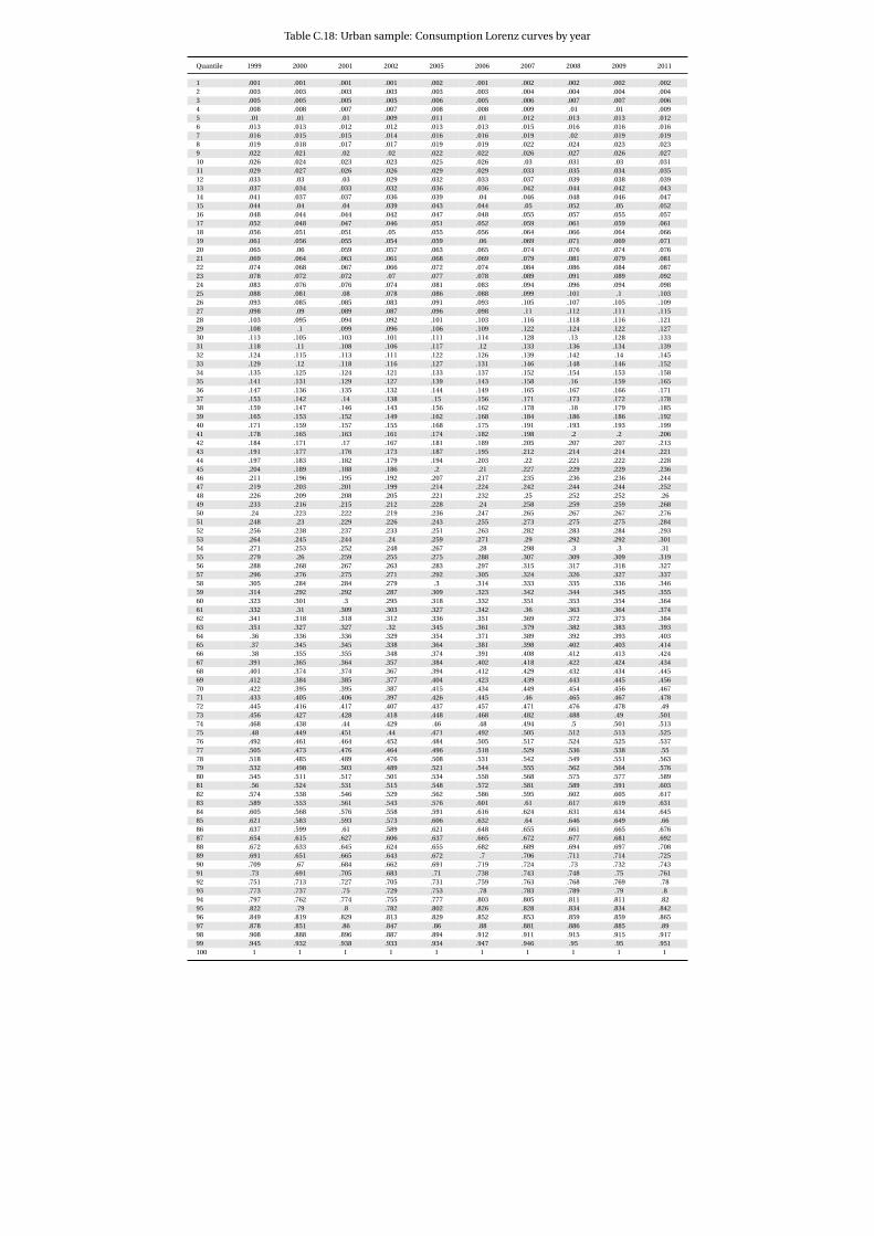
Table C.18: Urban sample: Consumption Lorenz curves by year

Quantile 1999 2000 2001 2002 2005 2006 2007 2008 2009 2011

1 .001 .001 .001 .001 .002 .001 .002 .002 .002 .0022 .003 .003 .003 .003 .003 .003 .004 .004 .004 .0043 .005 .005 .005 .005 .006 .005 .006 .007 .007 .0064 .008 .008 .007 .007 .008 .008 .009 .01 .01 .0095 .01 .01 .01 .009 .011 .01 .012 .013 .013 .0126 .013 .013 .012 .012 .013 .013 .015 .016 .016 .0167 .016 .015 .015 .014 .016 .016 .019 .02 .019 .0198 .019 .018 .017 .017 .019 .019 .022 .024 .023 .0239 .022 .021 .02 .02 .022 .022 .026 .027 .026 .02710 .026 .024 .023 .023 .025 .026 .03 .031 .03 .03111 .029 .027 .026 .026 .029 .029 .033 .035 .034 .03512 .033 .03 .03 .029 .032 .033 .037 .039 .038 .03913 .037 .034 .033 .032 .036 .036 .042 .044 .042 .04314 .041 .037 .037 .036 .039 .04 .046 .048 .046 .04715 .044 .04 .04 .039 .043 .044 .05 .052 .05 .05216 .048 .044 .044 .042 .047 .048 .055 .057 .055 .05717 .052 .048 .047 .046 .051 .052 .059 .061 .059 .06118 .056 .051 .051 .05 .055 .056 .064 .066 .064 .06619 .061 .056 .055 .054 .059 .06 .069 .071 .069 .07120 .065 .06 .059 .057 .063 .065 .074 .076 .074 .07621 .069 .064 .063 .061 .068 .069 .079 .081 .079 .08122 .074 .068 .067 .066 .072 .074 .084 .086 .084 .08723 .078 .072 .072 .07 .077 .078 .089 .091 .089 .09224 .083 .076 .076 .074 .081 .083 .094 .096 .094 .09825 .088 .081 .08 .078 .086 .088 .099 .101 .1 .10326 .093 .085 .085 .083 .091 .093 .105 .107 .105 .10927 .098 .09 .089 .087 .096 .098 .11 .112 .111 .11528 .103 .095 .094 .092 .101 .103 .116 .118 .116 .12129 .108 .1 .099 .096 .106 .109 .122 .124 .122 .12730 .113 .105 .103 .101 .111 .114 .128 .13 .128 .13331 .118 .11 .108 .106 .117 .12 .133 .136 .134 .13932 .124 .115 .113 .111 .122 .126 .139 .142 .14 .14533 .129 .12 .118 .116 .127 .131 .146 .148 .146 .15234 .135 .125 .124 .121 .133 .137 .152 .154 .153 .15835 .141 .131 .129 .127 .139 .143 .158 .16 .159 .16536 .147 .136 .135 .132 .144 .149 .165 .167 .166 .17137 .153 .142 .14 .138 .15 .156 .171 .173 .172 .17838 .159 .147 .146 .143 .156 .162 .178 .18 .179 .18539 .165 .153 .152 .149 .162 .168 .184 .186 .186 .19240 .171 .159 .157 .155 .168 .175 .191 .193 .193 .19941 .178 .165 .163 .161 .174 .182 .198 .2 .2 .20642 .184 .171 .17 .167 .181 .189 .205 .207 .207 .21343 .191 .177 .176 .173 .187 .195 .212 .214 .214 .22144 .197 .183 .182 .179 .194 .203 .22 .221 .222 .22845 .204 .189 .188 .186 .2 .21 .227 .229 .229 .23646 .211 .196 .195 .192 .207 .217 .235 .236 .236 .24447 .219 .203 .201 .199 .214 .224 .242 .244 .244 .25248 .226 .209 .208 .205 .221 .232 .25 .252 .252 .2649 .233 .216 .215 .212 .228 .24 .258 .259 .259 .26850 .24 .223 .222 .219 .236 .247 .265 .267 .267 .27651 .248 .23 .229 .226 .243 .255 .273 .275 .275 .28452 .256 .238 .237 .233 .251 .263 .282 .283 .284 .29353 .264 .245 .244 .24 .259 .271 .29 .292 .292 .30154 .271 .253 .252 .248 .267 .28 .298 .3 .3 .3155 .279 .26 .259 .255 .275 .288 .307 .309 .309 .31956 .288 .268 .267 .263 .283 .297 .315 .317 .318 .32757 .296 .276 .275 .271 .292 .305 .324 .326 .327 .33758 .305 .284 .284 .279 .3 .314 .333 .335 .336 .34659 .314 .292 .292 .287 .309 .323 .342 .344 .345 .35560 .323 .301 .3 .295 .318 .332 .351 .353 .354 .36461 .332 .31 .309 .303 .327 .342 .36 .363 .364 .37462 .341 .318 .318 .312 .336 .351 .369 .372 .373 .38463 .351 .327 .327 .32 .345 .361 .379 .382 .383 .39364 .36 .336 .336 .329 .354 .371 .389 .392 .393 .40365 .37 .345 .345 .338 .364 .381 .398 .402 .403 .41466 .38 .355 .355 .348 .374 .391 .408 .412 .413 .42467 .391 .365 .364 .357 .384 .402 .418 .422 .424 .43468 .401 .374 .374 .367 .394 .412 .429 .432 .434 .44569 .412 .384 .385 .377 .404 .423 .439 .443 .445 .45670 .422 .395 .395 .387 .415 .434 .449 .454 .456 .46771 .433 .405 .406 .397 .426 .445 .46 .465 .467 .47872 .445 .416 .417 .407 .437 .457 .471 .476 .478 .4973 .456 .427 .428 .418 .448 .468 .482 .488 .49 .50174 .468 .438 .44 .429 .46 .48 .494 .5 .501 .51375 .48 .449 .451 .44 .471 .492 .505 .512 .513 .52576 .492 .461 .464 .452 .484 .505 .517 .524 .525 .53777 .505 .473 .476 .464 .496 .518 .529 .536 .538 .5578 .518 .485 .489 .476 .508 .531 .542 .549 .551 .56379 .532 .498 .503 .489 .521 .544 .555 .562 .564 .57680 .545 .511 .517 .501 .534 .558 .568 .575 .577 .58981 .56 .524 .531 .515 .548 .572 .581 .589 .591 .60382 .574 .538 .546 .529 .562 .586 .595 .602 .605 .61783 .589 .553 .561 .543 .576 .601 .61 .617 .619 .63184 .605 .568 .576 .558 .591 .616 .624 .631 .634 .64585 .621 .583 .593 .573 .606 .632 .64 .646 .649 .6686 .637 .599 .61 .589 .621 .648 .655 .661 .665 .67687 .654 .615 .627 .606 .637 .665 .672 .677 .681 .69288 .672 .633 .645 .624 .655 .682 .689 .694 .697 .70889 .691 .651 .665 .643 .672 .7 .706 .711 .714 .72590 .709 .67 .684 .662 .691 .719 .724 .73 .732 .74391 .73 .691 .705 .683 .71 .738 .743 .748 .75 .76192 .751 .713 .727 .705 .731 .759 .763 .768 .769 .7893 .773 .737 .75 .729 .753 .78 .783 .789 .79 .894 .797 .762 .774 .755 .777 .803 .805 .811 .811 .8295 .822 .79 .8 .782 .802 .826 .828 .834 .834 .84296 .849 .819 .829 .813 .829 .852 .853 .859 .859 .86597 .878 .851 .86 .847 .86 .88 .881 .886 .885 .8998 .908 .888 .896 .887 .894 .912 .911 .915 .915 .91799 .945 .932 .938 .933 .934 .947 .946 .95 .95 .951100 1 1 1 1 1 1 1 1 1 1

47

Table C.20: Rural sample: Income Lorenz curves by year

Quantile 1999 2000 2001 2002 2003 2004 2005 2006 2007 2008 2009 2011

1 0 0 0 0 0 0 0 0 0 0 0 02 0 0 0 0 0 .001 0 0 0 .001 .001 .0013 .001 0 0 0 .001 .002 .001 .001 0 .001 .001 .0014 .001 .001 .001 .001 .001 .002 .001 .001 .001 .002 .002 .0025 .001 .001 .001 .001 .002 .003 .002 .001 .001 .002 .002 .0026 .002 .001 .002 .001 .003 .004 .003 .002 .002 .003 .003 .0037 .002 .002 .002 .002 .004 .005 .003 .002 .002 .004 .004 .0048 .003 .002 .003 .002 .005 .006 .004 .003 .003 .005 .005 .0059 .003 .002 .003 .003 .006 .007 .005 .004 .004 .006 .006 .00610 .004 .003 .004 .003 .008 .009 .006 .005 .004 .007 .007 .00811 .004 .004 .005 .004 .009 .01 .007 .005 .005 .008 .009 .00912 .005 .004 .006 .005 .011 .012 .008 .006 .006 .009 .01 .01113 .006 .005 .007 .005 .013 .013 .01 .007 .007 .01 .011 .01214 .006 .005 .008 .006 .015 .015 .011 .008 .008 .012 .013 .01415 .007 .006 .009 .007 .017 .017 .013 .01 .01 .013 .015 .01516 .008 .007 .01 .008 .019 .018 .014 .011 .011 .015 .016 .01717 .009 .008 .011 .009 .021 .02 .016 .012 .012 .016 .018 .01918 .01 .008 .013 .01 .023 .022 .018 .013 .014 .018 .02 .02119 .011 .009 .014 .012 .026 .024 .02 .015 .015 .02 .022 .02420 .012 .01 .016 .013 .028 .027 .022 .016 .017 .022 .024 .02621 .013 .011 .017 .015 .031 .029 .024 .018 .019 .024 .026 .02822 .014 .012 .019 .016 .034 .031 .026 .02 .021 .026 .028 .03123 .015 .013 .021 .018 .037 .034 .028 .021 .023 .028 .03 .03324 .017 .014 .023 .019 .04 .036 .03 .023 .025 .031 .033 .03625 .018 .015 .025 .021 .043 .039 .033 .025 .027 .033 .035 .03926 .02 .016 .027 .023 .046 .042 .035 .027 .029 .036 .038 .04227 .022 .018 .029 .025 .05 .045 .038 .029 .031 .039 .041 .04528 .023 .019 .031 .028 .053 .048 .041 .031 .034 .042 .044 .04929 .025 .02 .034 .03 .057 .051 .044 .034 .036 .045 .047 .05230 .027 .022 .036 .032 .06 .054 .047 .036 .039 .048 .05 .05631 .029 .023 .039 .035 .064 .058 .05 .039 .042 .052 .054 .05932 .031 .025 .041 .038 .068 .061 .053 .042 .044 .055 .058 .06333 .033 .027 .044 .04 .072 .065 .056 .045 .047 .059 .061 .06734 .036 .028 .047 .043 .077 .069 .059 .048 .05 .063 .065 .07135 .038 .03 .05 .046 .081 .073 .063 .051 .054 .067 .069 .07536 .041 .032 .053 .05 .085 .077 .067 .054 .057 .071 .073 .07937 .043 .034 .056 .053 .09 .082 .071 .058 .06 .075 .078 .08338 .046 .036 .06 .056 .094 .086 .074 .061 .064 .079 .082 .08839 .049 .038 .063 .06 .099 .091 .079 .065 .068 .084 .087 .09240 .052 .041 .067 .064 .103 .096 .083 .068 .072 .088 .092 .09741 .055 .043 .071 .067 .108 .101 .087 .072 .076 .093 .096 .10242 .058 .045 .075 .071 .113 .106 .092 .076 .08 .097 .101 .10743 .061 .048 .079 .076 .118 .111 .097 .08 .084 .102 .107 .11244 .064 .051 .084 .08 .124 .116 .101 .084 .089 .107 .112 .11745 .068 .054 .088 .084 .129 .122 .106 .089 .094 .112 .117 .12346 .072 .057 .093 .089 .134 .127 .111 .093 .099 .118 .123 .12847 .075 .06 .098 .094 .14 .133 .116 .097 .103 .123 .129 .13448 .079 .064 .103 .099 .145 .139 .122 .102 .108 .129 .135 .1449 .083 .067 .108 .104 .151 .145 .127 .107 .114 .135 .141 .14650 .088 .071 .113 .109 .157 .151 .133 .112 .119 .141 .147 .15251 .092 .075 .118 .115 .162 .157 .139 .117 .125 .147 .154 .15852 .096 .08 .124 .12 .168 .163 .145 .122 .13 .153 .16 .16553 .101 .084 .13 .126 .175 .17 .151 .128 .136 .16 .167 .17154 .106 .089 .135 .132 .181 .176 .158 .133 .143 .166 .174 .17855 .111 .093 .142 .138 .188 .183 .165 .139 .149 .173 .181 .18556 .117 .098 .148 .144 .194 .191 .172 .145 .155 .18 .189 .19257 .122 .104 .154 .151 .201 .198 .179 .151 .162 .187 .196 .258 .128 .109 .161 .158 .208 .205 .186 .158 .169 .195 .204 .20759 .135 .115 .168 .165 .216 .213 .193 .164 .176 .202 .213 .21560 .141 .121 .175 .172 .223 .221 .201 .171 .183 .21 .221 .22361 .147 .127 .183 .179 .231 .229 .209 .177 .19 .218 .23 .23162 .154 .133 .191 .187 .239 .237 .217 .184 .198 .226 .239 .2463 .161 .14 .198 .195 .247 .246 .225 .192 .206 .235 .247 .24864 .168 .147 .207 .203 .255 .254 .233 .199 .214 .244 .257 .25765 .176 .155 .215 .211 .263 .263 .242 .207 .222 .253 .266 .26666 .184 .162 .224 .22 .272 .272 .251 .214 .231 .262 .276 .27567 .192 .17 .233 .228 .28 .282 .26 .223 .239 .271 .286 .28568 .201 .178 .243 .238 .289 .291 .27 .231 .248 .281 .296 .29569 .209 .186 .252 .247 .298 .301 .279 .24 .258 .291 .307 .30570 .218 .195 .262 .257 .308 .312 .29 .249 .267 .302 .318 .31571 .227 .204 .272 .267 .317 .322 .3 .258 .277 .312 .329 .32572 .237 .213 .283 .277 .327 .332 .311 .268 .287 .323 .34 .33673 .247 .222 .294 .288 .338 .344 .322 .277 .298 .334 .352 .34874 .258 .233 .305 .299 .348 .355 .333 .288 .309 .345 .364 .35975 .269 .244 .316 .311 .359 .367 .345 .299 .32 .357 .377 .37176 .28 .255 .328 .323 .371 .378 .357 .31 .332 .369 .389 .38377 .292 .266 .34 .335 .382 .39 .369 .321 .345 .381 .402 .39678 .305 .279 .352 .347 .394 .403 .382 .334 .358 .394 .416 .40979 .318 .292 .365 .361 .407 .415 .395 .346 .371 .407 .43 .42280 .33 .305 .379 .374 .42 .428 .409 .359 .384 .421 .444 .43681 .345 .319 .393 .389 .433 .442 .424 .373 .399 .436 .458 .45182 .359 .333 .408 .403 .447 .456 .439 .387 .414 .45 .473 .46683 .374 .349 .423 .418 .461 .47 .455 .402 .43 .466 .49 .48284 .39 .364 .439 .435 .475 .485 .471 .418 .446 .482 .506 .49885 .407 .381 .456 .452 .491 .501 .488 .434 .463 .498 .523 .51586 .424 .399 .473 .47 .507 .518 .506 .452 .481 .516 .541 .53287 .442 .418 .492 .489 .523 .536 .525 .47 .5 .534 .56 .55188 .461 .437 .511 .509 .541 .554 .544 .49 .519 .553 .579 .56989 .481 .458 .531 .53 .56 .573 .564 .511 .539 .573 .6 .58990 .503 .48 .552 .553 .58 .594 .586 .533 .56 .594 .622 .6191 .526 .503 .575 .576 .602 .616 .608 .557 .584 .615 .646 .63292 .552 .528 .6 .601 .625 .639 .631 .583 .608 .638 .67 .65693 .58 .556 .627 .628 .652 .664 .656 .611 .635 .662 .696 .68194 .611 .586 .658 .657 .679 .691 .682 .64 .665 .687 .724 .70895 .646 .619 .691 .689 .709 .72 .711 .672 .699 .714 .754 .73796 .684 .657 .729 .725 .742 .752 .741 .708 .739 .743 .787 .7797 .729 .698 .771 .765 .782 .792 .776 .75 .784 .777 .825 .80798 .787 .752 .822 .814 .831 .839 .817 .801 .838 .819 .867 .85199 .864 .83 .888 .88 .893 .893 .875 .874 .902 .875 .915 .908100 1 1 1 1 1 1 1 1 1 1 1 1

48

Table C.21: Rural sample: Consumption Lorenz curves by year

Quantile 1999 2000 2001 2002 2005 2006 2007 2008 2009 2011

1 .001 .001 .001 .001 .001 .001 .001 .001 .001 .0012 .003 .003 .003 .002 .003 .003 .003 .003 .003 .0033 .004 .004 .005 .004 .005 .005 .006 .005 .005 .0054 .006 .006 .007 .006 .007 .007 .008 .007 .007 .0075 .008 .008 .009 .008 .009 .009 .01 .009 .009 .0096 .01 .01 .011 .01 .011 .012 .013 .011 .012 .0127 .013 .012 .014 .012 .013 .014 .016 .013 .015 .0148 .015 .014 .016 .015 .016 .017 .018 .016 .018 .0179 .017 .016 .019 .017 .018 .02 .021 .019 .02 .0210 .02 .018 .022 .02 .021 .022 .024 .021 .024 .02311 .023 .021 .025 .023 .024 .025 .028 .024 .027 .02612 .026 .024 .028 .026 .027 .028 .031 .027 .03 .0313 .029 .026 .031 .03 .03 .032 .034 .031 .034 .03314 .032 .029 .035 .033 .033 .035 .038 .034 .037 .03615 .035 .032 .038 .037 .037 .038 .041 .038 .041 .0416 .038 .035 .042 .04 .04 .042 .045 .041 .045 .04417 .041 .038 .045 .044 .044 .045 .049 .045 .049 .04818 .045 .042 .049 .048 .048 .049 .053 .049 .053 .05119 .048 .045 .053 .052 .051 .053 .057 .053 .058 .05620 .052 .048 .057 .056 .056 .057 .061 .057 .062 .0621 .055 .052 .061 .06 .06 .061 .065 .061 .067 .06422 .059 .056 .065 .064 .064 .065 .069 .066 .071 .06923 .063 .06 .069 .068 .069 .069 .073 .07 .076 .07324 .067 .063 .074 .073 .073 .073 .078 .075 .081 .07825 .071 .067 .078 .077 .078 .077 .083 .079 .086 .08326 .075 .072 .083 .082 .083 .082 .087 .084 .091 .08727 .08 .076 .087 .087 .088 .086 .092 .089 .096 .09228 .084 .08 .092 .091 .093 .091 .097 .094 .101 .09729 .089 .085 .097 .096 .098 .095 .102 .1 .106 .10330 .094 .089 .102 .101 .104 .1 .107 .105 .112 .10831 .098 .094 .108 .106 .109 .104 .113 .11 .117 .11332 .103 .099 .113 .112 .114 .109 .118 .116 .123 .11933 .108 .104 .119 .117 .12 .114 .124 .121 .129 .12534 .113 .109 .124 .122 .126 .119 .129 .127 .135 .13135 .118 .114 .13 .128 .132 .124 .135 .133 .141 .13736 .124 .119 .136 .133 .138 .129 .141 .139 .147 .14337 .129 .125 .141 .139 .144 .134 .147 .145 .153 .14938 .134 .131 .148 .145 .15 .14 .154 .151 .159 .15639 .14 .136 .154 .151 .156 .145 .16 .157 .166 .16240 .146 .142 .16 .157 .162 .151 .166 .163 .173 .16941 .152 .148 .166 .163 .169 .156 .173 .17 .179 .17642 .158 .154 .172 .169 .175 .162 .179 .176 .186 .18243 .164 .16 .179 .175 .182 .168 .186 .183 .193 .18944 .17 .167 .186 .182 .189 .174 .193 .19 .2 .19745 .176 .173 .192 .189 .196 .181 .2 .197 .207 .20446 .183 .18 .199 .195 .202 .187 .207 .204 .214 .21147 .19 .187 .206 .202 .209 .194 .214 .211 .222 .21948 .197 .194 .214 .209 .217 .201 .222 .219 .229 .22749 .204 .201 .221 .216 .224 .208 .229 .226 .236 .23550 .21 .209 .228 .224 .231 .215 .237 .234 .244 .24351 .218 .216 .236 .231 .239 .222 .244 .241 .252 .25152 .225 .224 .244 .239 .246 .229 .252 .249 .26 .25953 .233 .232 .251 .246 .254 .237 .26 .257 .268 .26754 .24 .24 .259 .254 .262 .245 .269 .265 .276 .27655 .248 .248 .267 .262 .27 .253 .277 .273 .285 .28556 .256 .256 .276 .27 .278 .261 .286 .282 .293 .29457 .264 .264 .284 .278 .286 .269 .295 .29 .302 .30258 .272 .273 .293 .287 .295 .278 .304 .299 .311 .31259 .281 .282 .302 .295 .304 .287 .313 .308 .32 .32160 .289 .291 .311 .304 .312 .295 .322 .317 .329 .33161 .298 .3 .32 .313 .321 .304 .331 .326 .339 .34162 .307 .309 .329 .322 .33 .313 .341 .336 .348 .3563 .316 .319 .339 .331 .34 .323 .351 .346 .358 .36164 .325 .328 .349 .341 .349 .332 .361 .356 .368 .37165 .335 .338 .359 .35 .359 .342 .371 .366 .378 .38266 .345 .348 .369 .36 .369 .352 .382 .376 .389 .39267 .355 .359 .38 .37 .379 .362 .393 .386 .399 .40368 .365 .369 .39 .38 .389 .372 .403 .397 .41 .41469 .376 .38 .401 .39 .4 .383 .415 .408 .421 .42670 .386 .391 .413 .401 .411 .393 .426 .42 .432 .43771 .397 .403 .424 .411 .422 .404 .437 .431 .444 .44972 .408 .415 .436 .422 .433 .416 .449 .443 .455 .46173 .419 .426 .447 .434 .445 .427 .461 .455 .467 .47374 .431 .439 .459 .445 .457 .439 .473 .467 .479 .48575 .443 .451 .472 .457 .469 .451 .485 .479 .491 .49876 .456 .464 .484 .468 .481 .463 .498 .492 .503 .51177 .469 .478 .497 .481 .493 .476 .511 .505 .516 .52478 .482 .491 .51 .493 .506 .489 .524 .518 .529 .53779 .496 .505 .524 .506 .52 .502 .538 .532 .542 .5580 .51 .519 .537 .519 .533 .516 .552 .546 .556 .56481 .524 .534 .551 .533 .547 .529 .565 .56 .57 .57982 .539 .549 .566 .547 .562 .544 .579 .575 .584 .59383 .554 .564 .581 .561 .576 .558 .594 .59 .599 .60884 .57 .58 .596 .576 .592 .574 .609 .606 .614 .62385 .586 .596 .612 .592 .607 .59 .625 .622 .63 .63986 .603 .613 .629 .608 .624 .606 .64 .639 .646 .65587 .62 .63 .646 .625 .64 .623 .656 .656 .662 .67288 .638 .649 .663 .643 .657 .641 .673 .674 .679 .68989 .657 .667 .681 .661 .675 .66 .691 .692 .697 .70690 .677 .687 .7 .68 .693 .679 .709 .712 .715 .72591 .698 .707 .719 .7 .712 .7 .728 .732 .734 .74492 .72 .728 .74 .721 .733 .721 .748 .753 .754 .76493 .745 .751 .761 .744 .755 .743 .77 .775 .776 .78594 .77 .775 .784 .767 .778 .768 .792 .798 .799 .80795 .797 .801 .809 .792 .803 .794 .816 .822 .823 .8396 .825 .828 .835 .819 .829 .822 .843 .849 .849 .85597 .855 .859 .866 .85 .859 .855 .873 .876 .878 .88298 .89 .893 .901 .884 .893 .892 .907 .907 .909 .91399 .932 .934 .942 .927 .934 .935 .945 .945 .946 .95100 1 1 1 1 1 1 1 1 1 1

49

Table C.16: National sample: Gains in income and consumption shares by quantile


1 110.11 77.5 272.96 23.12 42.41 75.332 132.87 78.36 315.35 23.51 45.73 79.993 138.89 93.79 362.95 23.68 53.09 89.344 152.55 77.3 347.78 21.62 51.87 84.75 174.72 60.97 342.23 22.26 45.04 77.336 161.02 68.05 338.64 27.19 38.05 75.597 164.43 73.52 358.83 29.59 37.24 77.858 158.63 71.97 344.76 34.79 34.71 81.589 141.22 69.35 308.5 35.75 32.78 80.2510 123.57 69.61 279.2 34.97 31.31 77.2211 106.24 68 246.49 31.78 29.51 70.6712 103.46 65.67 237.06 30.63 30.37 70.3113 100.73 61.1 223.39 29.15 29.14 66.7814 98.36 55.73 208.91 27.57 31.05 67.1715 92.6 55.1 198.72 25.54 32.15 65.8916 90.92 49.89 186.18 24.31 32.53 64.7517 89.48 45.58 175.85 25.1 33.05 66.4518 75.82 45.46 155.75 17.1 33.5 56.3319 79.03 45.24 160.02 17.78 33.21 56.920 66.75 42.28 137.25 15.37 32.38 52.7321 62.04 44.16 133.59 13.95 32.01 50.4222 52.47 42.75 117.65 16.11 30.93 52.0323 44.97 42.85 107.09 13.83 31.28 49.4424 39.09 44.22 100.6 11.86 31.15 46.725 39.2 38.9 93.34 11.34 31.21 46.0926 32.83 40.53 86.67 11.03 29.78 44.127 29.47 39.44 80.53 8.53 30.13 41.2328 27.22 39.47 77.43 7.42 29.34 38.9329 26.37 38.6 75.15 4.95 29.28 35.6830 20.36 40.6 69.23 5.17 27.66 34.2631 20.9 40.72 70.13 5.44 26.93 33.8432 22.18 41.99 73.48 3.61 26.73 31.3133 17.85 39.91 64.88 4.37 25.96 31.4734 17.25 41.42 65.82 2.64 25.09 28.435 16.33 35.63 57.78 3.2 25.37 29.3736 13.91 38.14 57.35 4.14 24.13 29.2737 12.39 35.83 52.66 4.77 23.68 29.5838 8.58 36.17 47.86 3.23 22.4 26.3639 9.34 35.93 48.62 4.66 21.44 27.0940 6.7 36.6 45.76 4.05 19.84 24.741 7.84 35.59 46.22 2.91 20.87 24.3942 5.88 34.16 42.05 2.99 19.71 23.2843 5.69 34.42 42.07 4.17 18.3 23.2344 4.13 32.64 38.12 3.19 18.71 22.4945 4.89 32.59 39.07 3.9 17.98 22.5846 2.54 33.4 36.79 .64 18.32 19.0747 2.37 32.88 36.02 .61 17.65 18.3748 2.36 32.51 35.64 .04 17.94 17.9949 .7 29.5 30.41 .02 17.31 17.3350 2.73 29.38 32.91 1.23 16.38 17.8151 -.03 27.47 27.43 .04 15.94 1652 .51 27.31 27.96 .61 15.99 16.6953 .51 25.82 26.45 .87 14.31 15.354 1.02 25.19 26.46 -.7 14.53 13.7255 -.77 24.11 23.15 -2.02 14.5 12.1856 -.12 23.24 23.09 -1.54 13.67 11.9257 -1.32 21.95 20.34 -1.72 13.49 11.5358 -2.36 22.69 19.79 -1.06 12.55 11.3559 -2.45 21.88 18.9 -3.57 12.79 8.7660 -2.38 21.5 18.61 -2.06 12.34 10.0261 -2.28 21.26 18.5 -2.95 11.82 8.5262 -3.73 21.3 16.78 -3.3 11.22 7.5563 -4.14 19.76 14.8 -3.75 9.9 5.7864 -3.48 18.78 14.65 -3.13 9 5.665 -3.73 18.32 13.9 -2.34 8.13 5.666 -5.79 19.23 12.33 -1.69 6.63 4.8267 -4.55 19.48 14.04 -2.24 6.19 3.8168 -3.75 15.69 11.35 -.84 3.44 2.5769 -5.28 17.34 11.14 -.99 4.01 2.9870 -7.26 17.06 8.57 -.6 3.6 2.9871 -6.95 16.24 8.16 -.87 3.07 2.1772 -5.22 13.64 7.71 -2.51 3.61 1.0273 -6.79 15.16 7.34 -3.09 3.37 .1774 -5.66 14.82 8.32 -4.48 2.98 -1.6475 -5.02 13.04 7.37 -4.16 1.57 -2.6676 -2.42 10.4 7.74 -4.77 1.67 -3.1777 -6.01 10.8 4.13 -4.72 1.04 -3.7378 -5.03 8.86 3.38 -4.73 .37 -4.3779 -8.5 9.61 .29 -4.09 .71 -3.4280 -6.83 8.77 1.34 -2.17 -.59 -2.7581 -7.18 7.04 -.65 -3.24 -1.95 -5.1382 -6.26 6.3 -.35 -2.54 -2.04 -4.5283 -6.29 4.14 -2.41 -2.74 -2.79 -5.4584 -6.88 2.66 -4.41 -6.5 -2.25 -8.685 -7.45 3.44 -4.28 -4.32 -4.21 -8.3586 -7.01 .67 -6.39 -6.06 -2.96 -8.8487 -6.29 -1.41 -7.61 -8.39 -4.66 -12.6688 -5.87 -1.28 -7.07 -6.13 -5.76 -11.5489 -6.12 -1.8 -7.8 -7.53 -5.9 -12.9990 -6.33 -4.08 -10.15 -8.39 -4.52 -12.5391 -7.22 -3.89 -10.83 -5.56 -6.67 -11.8692 -7.07 -5.67 -12.34 -7.8 -8.84 -15.9693 -6.25 -9.22 -14.89 -5.86 -9.53 -14.8394 -6.07 -12.73 -18.03 -5.26 -12 -16.6395 -6.28 -13.66 -19.08 -2.18 -15 -16.8596 -2.81 -17.06 -19.39 -4.61 -16.78 -20.6197 1 -18.95 -18.14 -3.85 -19.47 -22.5798 3.4 -23.8 -21.21 3.81 -23.7 -20.7999 -5.09 -23.09 -27.01 4.4 -23.45 -20.08100 8.42 -41.75 -36.84 11.78 -29.06 -20.7

50

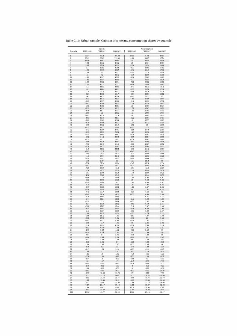
Table C.19: Urban sample: Gains in income and consumption shares by quantile


1 69.57 68.9 186.42 37.55 8.74 49.572 28.25 66.85 113.98 3.03 14.27 17.743 16.09 41.82 64.65 .55 15.45 16.084 7.43 37.32 47.52 .28 20.54 20.875 3.65 35.98 40.94 -2.96 23.54 19.886 3.7 30.82 35.66 -3.31 21.65 17.627 4.29 33.35 39.07 -1.96 19.45 17.128 2.34 37 40.21 -7.15 23.3 14.499 .5 42 42.72 -5.78 22.68 15.5910 4.86 40.47 47.29 -8.96 25.05 13.8511 2.46 38.54 41.95 -6.77 22.55 14.2612 2.96 39.22 43.34 -7.28 22.82 13.8813 2.11 40.15 43.1 -3.96 21.48 16.6714 -1.1 44.52 42.93 -4.41 21.13 15.815 .04 44.04 44.11 -2.57 20.56 17.4616 -2.4 45.6 42.11 -1.98 20.16 17.7817 -8.21 45.65 33.7 -1.81 21.01 18.8218 .68 41.32 42.28 -3.42 20.11 1619 -1.32 43.12 41.23 1.26 17.56 19.0320 -3.09 40.57 36.22 -1.3 18.93 17.3821 -1.81 40.88 38.33 1.74 17.38 19.4222 -5.05 40.93 33.81 .25 20.07 20.3723 -5.92 43.92 35.39 1.75 17.67 19.7224 -4.48 41.71 35.37 -.26 17.63 17.3225 -3.79 41 35.66 -.41 17.79 17.3126 -5.92 40.19 31.9 -.6 16.03 15.3327 -4.03 39.75 34.11 -1.22 18.97 17.5128 -5.02 39.69 32.68 -.8 17.77 16.8329 -4.79 38.89 32.23 -.16 17.73 17.5430 -6.55 39.62 30.47 -1.58 17 15.1531 -7.73 38.71 27.99 -2.27 17.1 14.4532 -9.42 40.88 27.61 -1.58 17.49 15.6433 -5.93 37.95 29.78 -.82 16.72 15.7734 -7.55 34.85 24.67 -1.38 15.83 14.2435 -6.92 34.5 25.19 -2.17 15.64 13.1336 -7.32 33.71 23.93 -2.34 16.61 13.8937 -6.99 32.26 23.02 -2.02 16.85 14.4838 -7.76 32.15 21.9 -2.89 15.87 12.5239 -6.78 31.77 22.83 -4.39 16.64 11.5240 -5.3 31.65 24.68 -1.09 15.12 13.8741 -5.65 27.6 20.39 -3.41 16.92 12.9342 -7.65 29.1 19.23 -1.23 14.08 12.6943 -4.9 27.71 21.46 -2.86 14.56 11.2844 -6.19 27.41 19.52 -3.04 14.66 11.1745 -6.18 26.84 19 -5.21 14.78 8.846 -7.58 27.94 18.24 -2.47 15.18 12.3447 -6.07 25.81 18.17 -2.73 12.04 8.9848 -7.25 25.39 16.3 -1.54 12.8 11.0749 -5.9 25.12 17.74 -.13 10.44 10.350 -5.91 25.68 18.26 -.73 11.06 10.2551 -4.56 23.05 17.45 .13 10.44 10.5952 -3.66 23.6 19.08 -.86 9.96 9.0153 -6.22 23.96 16.26 .28 9.52 9.8354 -6.24 23.84 16.1 1.06 8.66 9.8155 -5.4 23.21 16.55 .28 7.95 8.2656 -5.17 22.09 15.78 1.39 6.57 8.0657 -6.16 22.99 15.42 .84 7.31 8.2258 -7.42 22.7 13.59 -1.27 7.56 6.259 -5.42 21.16 14.59 -1.31 6.89 5.4960 -5.28 21.04 14.64 -2.1 6.41 4.1761 -5.41 21.24 14.68 -2.5 6.92 4.2462 -2.59 17.1 14.06 -3.51 7.62 3.8463 -3.24 18.36 14.52 -3.83 6.59 2.5164 -2.08 17.89 15.44 -5.6 7.47 1.4565 -4.45 18.83 13.54 -3.19 6.34 2.9566 -2.6 15.57 12.56 -1.63 5.39 3.6767 -.93 13.79 12.74 -2.51 4.75 2.1268 -5.98 14.72 7.86 -2.87 4.37 1.3869 -5.08 15.52 9.64 -1.16 4.8 3.5970 -2.93 12.21 8.93 -1.29 3.61 2.2771 -6.88 12.7 4.95 .08 2.85 2.9472 -5.6 12.54 6.24 -2.36 3.63 1.1973 -2.52 9.79 7.02 .59 1.81 2.4174 -4.59 9.62 4.58 -2.26 2.42 .1175 -3.14 8.74 5.32 -3 3.04 -.0476 -2.51 5.4 2.75 -1.75 1.83 .0577 -2.26 5.63 3.25 -3.19 1.5 -1.7378 -2.11 4.48 2.28 -4.82 1.42 -3.4779 -3.36 5.96 2.4 -5.79 1.92 -3.9880 -.09 3.46 3.37 -5.31 2.45 -381 -2.78 3.2 .33 -6.45 1.22 -5.3182 -1.41 1.24 -.18 -4.11 -1.44 -5.4983 -.86 .47 -.4 -6.12 1.15 -5.0384 1.06 .4 1.46 -4.3 -1.03 -5.2985 -2.56 -.63 -3.18 -5.51 -.53 -6.0186 -2.54 .2 -2.35 -6.69 .82 -5.9287 .26 -.97 -.71 -4.47 -3.31 -7.6388 -5.95 -1.04 -6.94 -3.79 -4.16 -7.889 -2.16 -3.95 -6.03 -4 -4.76 -8.5790 -.43 -6.19 -6.59 -.91 -5.12 -5.9891 -2.03 -7.91 -9.77 -4.32 -6.93 -10.9592 -1.95 -10.03 -11.78 .37 -8.17 -7.8393 3.5 -12.24 -9.17 -1.7 -10.44 -11.9694 -1.93 -11.64 -13.35 -1.05 -11.76 -12.6895 4.05 -15.63 -12.21 -1.73 -13.05 -14.5696 8.4 -18.8 -11.98 1.34 -17.18 -16.0897 7.87 -23.17 -17.12 8.92 -19.27 -12.0898 -.99 -19.3 -20.1 13.74 -18.86 -7.7199 -1.52 -23.22 -24.38 8.36 -16.88 -9.94100 18.52 -41.77 -30.99 18.66 -25.14 -11.17

51

Table C.22: Rural sample: Gains in income and consumption shares by quantile


1 28.15 71.52 119.8 9.17 4.39 13.962 51.47 24.06 87.92 4.5 2.74 7.373 44.36 20.26 73.61 6.58 2.84 9.614 66.96 14.63 91.39 7.73 5.62 13.785 55.15 29.43 100.81 5.09 9.62 15.26 66.2 31.7 118.88 8 8.58 17.277 66.9 36.79 128.3 5.88 13.23 19.888 75.13 32.24 131.59 6.78 14.45 22.219 66.97 26.04 110.46 1.52 17.91 19.710 78.61 21.26 116.58 4.84 13.79 19.2911 96.61 17.51 131.04 .07 12.93 1312 92.21 11.99 115.27 4.08 10.42 14.9313 105.33 8.06 121.89 3.07 10.08 13.4614 89.25 9.12 106.51 4.93 4.54 9.6915 87.95 15.31 116.72 9.62 5.67 15.8316 93.06 15.38 122.76 9.48 3.57 13.3917 88.9 20.51 127.64 9.45 5.2 15.1418 89.33 22.13 131.23 11.52 2.51 14.3219 88.82 23.05 132.34 10.78 3.99 15.220 92.57 20.27 131.6 14.01 3.25 17.7221 80.29 19.1 114.72 17.49 3.95 22.1322 80.39 17.02 111.08 15.72 .17 15.9123 76.89 15.81 104.85 13.82 1.44 15.4524 71.85 18.42 103.51 15.72 .87 16.7325 70.12 19.05 102.53 18.04 -.32 17.6626 64.86 15.71 90.76 15.63 -.07 15.5527 48.39 19.14 76.79 13.02 .39 13.4628 53.89 21.71 87.29 13.43 -.33 13.0629 59.96 17.7 88.28 13.91 -1.22 12.5230 47.25 20.64 77.64 13.55 1.07 14.7731 48.76 19.89 78.34 12.76 1.32 14.2632 44.68 20.93 74.96 13.95 1.07 15.1733 50.13 13.76 70.79 15.9 1.36 17.4834 48.07 18.99 76.19 12.37 1.74 14.3235 50.52 12.59 69.47 11.76 3.76 15.9736 42.15 17.36 66.83 12.09 3.13 15.637 48.42 12.45 66.91 10.73 6.62 18.0638 48.29 10.57 63.96 16.04 5.37 22.2739 46.22 11.51 63.05 6.04 4.95 11.2940 51.36 9.31 65.44 14.18 5.06 19.9541 48.77 9.62 63.09 9.37 5.32 15.1942 48.15 9.54 62.28 11.56 4.52 16.643 43.6 7.51 54.38 9.22 6.36 16.1644 38.69 10.1 52.71 6.25 5.94 12.5745 31.52 9.5 44.01 6.55 6.4 13.3746 39.76 10.8 54.85 6.47 6.23 13.1147 40.1 9.48 53.38 4.03 9.21 13.6248 34.54 11.08 49.46 5.18 6.62 12.1449 33.4 11.75 49.07 4.63 8.06 13.0750 35.75 6.62 44.74 5.2 9.65 15.3551 33.76 9.51 46.48 1.97 8.71 10.8652 39.75 5.8 47.86 3.38 9.64 13.3453 33.37 2.19 36.28 4.37 10.09 14.954 29.76 4.21 35.22 1.71 8.94 10.855 30.7 3.63 35.45 2.96 7.35 10.5356 29.64 1.88 32.07 3.3 10.22 13.8657 24.85 3.18 28.83 2.94 7.14 10.358 22.18 4.9 28.16 3.8 9.92 14.0959 17.8 5.11 23.82 4.33 6.44 11.0560 22.09 5.89 29.28 3.49 10.06 13.961 18.25 7.79 27.46 3.7 8.55 12.5762 18.14 5.22 24.3 .81 8.96 9.8463 19.43 4.23 24.48 .45 11.62 12.1264 17.08 2.7 20.25 4.22 6.73 11.2465 15.21 4.67 20.59 -1.63 9.46 7.6866 14.2 1.59 16.02 1.21 6.01 7.2967 14.45 3.47 18.43 2.06 7.98 10.268 8.69 2.88 11.82 .02 8.51 8.5469 15.03 3.84 19.45 .48 7.78 8.370 12.29 -.13 12.15 1.39 6.23 7.771 12.28 3.08 15.74 3.48 1.77 5.3172 13.11 3.52 17.09 1.31 6.8 8.273 4.81 1.83 6.72 2.44 5.05 7.6174 7.95 -1.27 6.58 2.4 5.96 8.5175 4.26 3.85 8.27 -2.07 5.01 2.8476 6.04 1.13 7.24 -1.99 2.34 .377 2.02 2.48 4.55 -2.15 5.85 3.5778 -1.05 3.19 2.1 -4.02 2.92 -1.2279 4.2 -1.42 2.72 -1.52 -2.02 -3.5180 13.23 .67 13.98 -4.59 5.41 .5781 4.08 -1.27 2.76 -2.12 2.7 .5282 7.5 -.03 7.47 -.94 .31 -.6383 3.24 -1.13 2.08 -3.1 .11 -2.9984 1.35 1.85 3.22 -3.29 .51 -2.885 2.43 -3.64 -1.3 -3.6 .29 -3.3286 .26 -.38 -.12 -3.28 -1.64 -4.8787 3.83 -2.03 1.73 -5.77 .18 -5.688 5.79 -2.49 3.16 -6.03 .36 -5.6989 1.51 -3.25 -1.79 -7.35 1.28 -6.1790 -2.82 -2.02 -4.79 -6.63 .53 -6.1491 -7.83 .62 -7.26 -8.18 -1.65 -9.6992 -9.05 1.3 -7.87 -8.23 -1.54 -9.6393 -11.28 1.89 -9.61 -11.92 -4.36 -15.7694 -17.28 3.31 -14.54 -5.88 -7.05 -12.5195 -15.8 2.25 -13.9 -6.37 -5.8 -11.896 -18.65 7.07 -12.9 -5.98 -5.28 -10.9497 -22.42 5.87 -17.86 -3.81 -7.62 -11.1398 -30.28 6.89 -25.47 -3.71 -7.76 -11.1999 -25.22 -1.58 -26.4 -1.95 -11.12 -12.86100 -7.7 -26.31 -31.98 -2.15 -24.63 -26.25

52

5SFOET JO JODPNF BOE DPOTVNQUJPO JOFRVBMJUZ JO … · cilios Argentina 1974,1980,1986-2010 Encuesta...

Documents

Transcript of 5SFOET JO JODPNF BOE DPOTVNQUJPO JOFRVBMJUZ JO … · cilios Argentina 1974,1980,1986-2010 Encuesta...